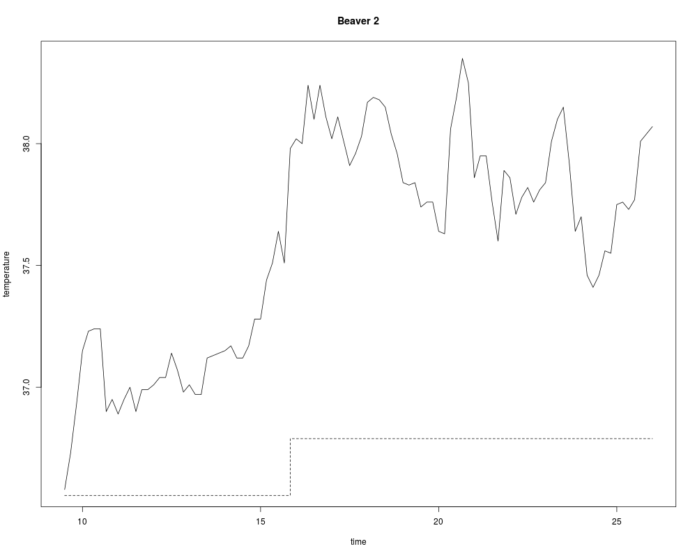
Body Temperature Series of Beaver 2

Description

Reynolds (1994) describes a small part of a study of the long-term temperature dynamics of beaver Castor canadensis in north-central Wisconsin. Body temperature was measured by telemetry every 10 minutes for four females, but data from a one period of less than a day for each of two animals is used there.

Usage

beav2

Format

The beav2 data frame has 100 rows and 4 columns. This data frame contains the following columns:

day

Day of observation (in days since the beginning of 1990), November 3–4.

time

Time of observation, in the form 0330 for 3.30am.

temp

Measured body temperature in degrees Celsius.

activ

Indicator of activity outside the retreat.

Source

P. S. Reynolds (1994) Time-series analyses of beaver body temperatures. Chapter 11 of Lange, N., Ryan, L., Billard, L., Brillinger, D., Conquest, L. and Greenhouse, J. eds (1994) Case Studies in Biometry. New York: John Wiley and Sons.

References

Venables, W. N. and Ripley, B. D. (2002) Modern Applied Statistics with S. Fourth edition. Springer.

See Also

beav1

Examples

attach(beav2)
beav2$hours <- 24*(day-307) + trunc(time/100) + (time%%100)/60
plot(beav2$hours, beav2$temp, type = "l", xlab = "time",
   ylab = "temperature", main = "Beaver 2")
usr <- par("usr"); usr[3:4] <- c(-0.2, 8); par(usr = usr)
lines(beav2$hours, beav2$activ, type = "s", lty = 2)

temp <- ts(temp, start = 8+2/3, frequency = 6)
activ <- ts(activ, start = 8+2/3, frequency = 6)
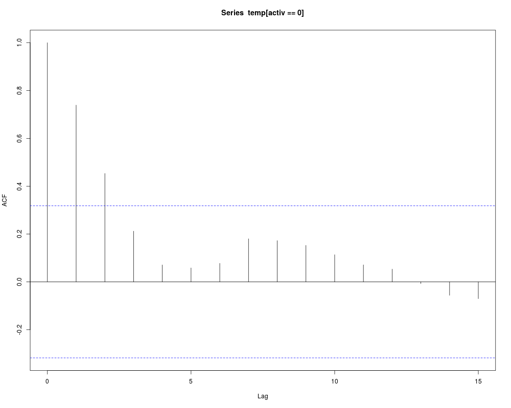
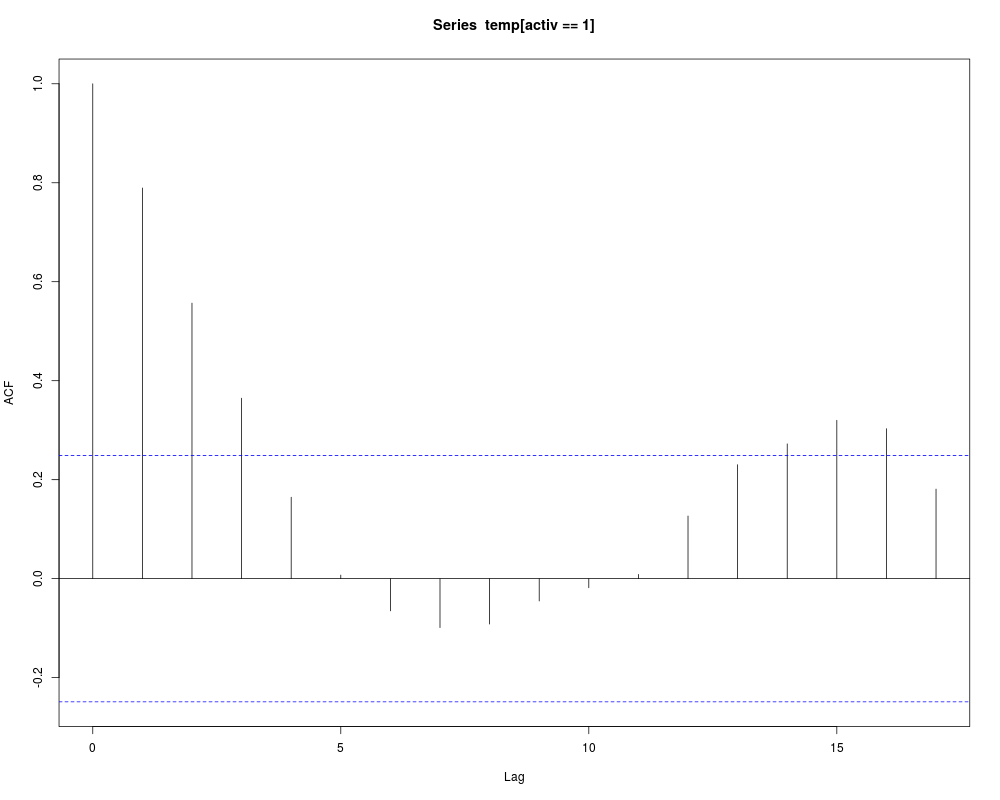
acf(temp[activ == 0]); acf(temp[activ == 1]) # also look at PACFs
ar(temp[activ == 0]); ar(temp[activ == 1])

arima(temp, order = c(1,0,0), xreg = activ)
dreg <- cbind(sin = sin(2*pi*beav2$hours/24), cos = cos(2*pi*beav2$hours/24))
arima(temp, order = c(1,0,0), xreg = cbind(active=activ, dreg))

library(nlme) # for gls and corAR1
beav2.gls <- gls(temp ~ activ, data = beav2, corr = corAR1(0.8),
                 method = "ML")
summary(beav2.gls)
summary(update(beav2.gls, subset = 6:100))
detach("beav2"); rm(temp, activ)

Results

R version 3.3.1 (2016-06-21) -- "Bug in Your Hair"
Copyright (C) 2016 The R Foundation for Statistical Computing
Platform: x86_64-pc-linux-gnu (64-bit)

R is free software and comes with ABSOLUTELY NO WARRANTY.
You are welcome to redistribute it under certain conditions.
Type 'license()' or 'licence()' for distribution details.

R is a collaborative project with many contributors.
Type 'contributors()' for more information and
'citation()' on how to cite R or R packages in publications.

Type 'demo()' for some demos, 'help()' for on-line help, or
'help.start()' for an HTML browser interface to help.
Type 'q()' to quit R.

> library(MASS)
> png(filename="/home/ddbj/snapshot/RGM3/R_CC/result/MASS/beav2.Rd_%03d_medium.png", width=480, height=480)
> ### Name: beav2
> ### Title: Body Temperature Series of Beaver 2
> ### Aliases: beav2
> ### Keywords: datasets
> 
> ### ** Examples
> 
> attach(beav2)
> beav2$hours <- 24*(day-307) + trunc(time/100) + (time%%100)/60
> plot(beav2$hours, beav2$temp, type = "l", xlab = "time",
+    ylab = "temperature", main = "Beaver 2")
> usr <- par("usr"); usr[3:4] <- c(-0.2, 8); par(usr = usr)
> lines(beav2$hours, beav2$activ, type = "s", lty = 2)
> 
> temp <- ts(temp, start = 8+2/3, frequency = 6)
> activ <- ts(activ, start = 8+2/3, frequency = 6)
> acf(temp[activ == 0]); acf(temp[activ == 1]) # also look at PACFs
> ar(temp[activ == 0]); ar(temp[activ == 1])

Call:
ar(x = temp[activ == 0])

Coefficients:
     1  
0.7392  

Order selected 1  sigma^2 estimated as  0.02011

Call:
ar(x = temp[activ == 1])

Coefficients:
     1  
0.7894  

Order selected 1  sigma^2 estimated as  0.01792
> 
> arima(temp, order = c(1,0,0), xreg = activ)

Call:
arima(x = temp, order = c(1, 0, 0), xreg = activ)

Coefficients:
         ar1  intercept   activ
      0.8733    37.1920  0.6139
s.e.  0.0684     0.1187  0.1381

sigma^2 estimated as 0.01518:  log likelihood = 66.78,  aic = -125.55
> dreg <- cbind(sin = sin(2*pi*beav2$hours/24), cos = cos(2*pi*beav2$hours/24))
> arima(temp, order = c(1,0,0), xreg = cbind(active=activ, dreg))

Call:
arima(x = temp, order = c(1, 0, 0), xreg = cbind(active = activ, dreg))

Coefficients:
         ar1  intercept  active  dreg.sin  dreg.cos
      0.7905    37.1674  0.5322    -0.282    0.1201
s.e.  0.0681     0.0939  0.1282     0.105    0.0997

sigma^2 estimated as 0.01434:  log likelihood = 69.83,  aic = -127.67
> 
> library(nlme) # for gls and corAR1
> beav2.gls <- gls(temp ~ activ, data = beav2, corr = corAR1(0.8),
+                  method = "ML")
> summary(beav2.gls)
Generalized least squares fit by maximum likelihood
  Model: temp ~ activ 
  Data: beav2 
        AIC       BIC   logLik
  -125.5505 -115.1298 66.77523

Correlation Structure: AR(1)
 Formula: ~1 
 Parameter estimate(s):
      Phi 
0.8731771 

Coefficients:
               Value Std.Error  t-value p-value
(Intercept) 37.19195 0.1131328 328.7460       0
activ        0.61418 0.1087286   5.6487       0

 Correlation: 
      (Intr)
activ -0.582

Standardized residuals:
        Min          Q1         Med          Q3         Max 
-2.42080780 -0.61510520 -0.03573836  0.81641138  2.15153499 

Residual standard error: 0.2527856 
Degrees of freedom: 100 total; 98 residual
> summary(update(beav2.gls, subset = 6:100))
Generalized least squares fit by maximum likelihood
  Model: temp ~ activ 
  Data: beav2 
  Subset: 6:100 
       AIC       BIC   logLik
  -124.981 -114.7654 66.49048

Correlation Structure: AR(1)
 Formula: ~1 
 Parameter estimate(s):
      Phi 
0.8380448 

Coefficients:
               Value  Std.Error  t-value p-value
(Intercept) 37.25001 0.09634047 386.6496       0
activ        0.60277 0.09931904   6.0690       0

 Correlation: 
      (Intr)
activ -0.657

Standardized residuals:
       Min         Q1        Med         Q3        Max 
-2.0231494 -0.8910348 -0.1497564  0.7640939  2.2719468 

Residual standard error: 0.2188542 
Degrees of freedom: 95 total; 93 residual
> detach("beav2"); rm(temp, activ)
> 
> 
> 
> 
> 
> dev.off()
null device 
          1 
>