R Graphical Manual

Browse All

Last data update: 2014.03.03

R: Ridge Regression

lm.ridge

R Documentation

Ridge Regression

Description

Fit a linear model by ridge regression.

Usage

lm.ridge(formula, data, subset, na.action, lambda = 0, model = FALSE,
         x = FALSE, y = FALSE, contrasts = NULL, ...)

Arguments

`formula`	a formula expression as for regression models, of the form `response ~ predictors`. See the documentation of `formula` for other details. `offset` terms are allowed.
`data`	an optional data frame in which to interpret the variables occurring in `formula`.
`subset`	expression saying which subset of the rows of the data should be used in the fit. All observations are included by default.
`na.action`	a function to filter missing data.
`lambda`	A scalar or vector of ridge constants.
`model`	should the model frame be returned? Not implemented.
`x`	should the design matrix be returned? Not implemented.
`y`	should the response be returned? Not implemented.
`contrasts`	a list of contrasts to be used for some or all of factor terms in the formula. See the `contrasts.arg` of `model.matrix.default`.
`...`	additional arguments to `lm.fit`.

Details

If an intercept is present in the model, its coefficient is not penalized. (If you want to penalize an intercept, put in your own constant term and remove the intercept.)

Value

A list with components

`coef`	matrix of coefficients, one row for each value of `lambda`. Note that these are not on the original scale and are for use by the `coef` method.
`scales`	scalings used on the X matrix.
`Inter`	was intercept included?
`lambda`	vector of lambda values
`ym`	mean of `y`
`xm`	column means of `x` matrix
`GCV`	vector of GCV values
`kHKB`	HKB estimate of the ridge constant.
`kLW`	L-W estimate of the ridge constant.

References

Brown, P. J. (1994) Measurement, Regression and Calibration Oxford.

Examples

longley # not the same as the S-PLUS dataset
names(longley)[1] <- "y"
lm.ridge(y ~ ., longley)
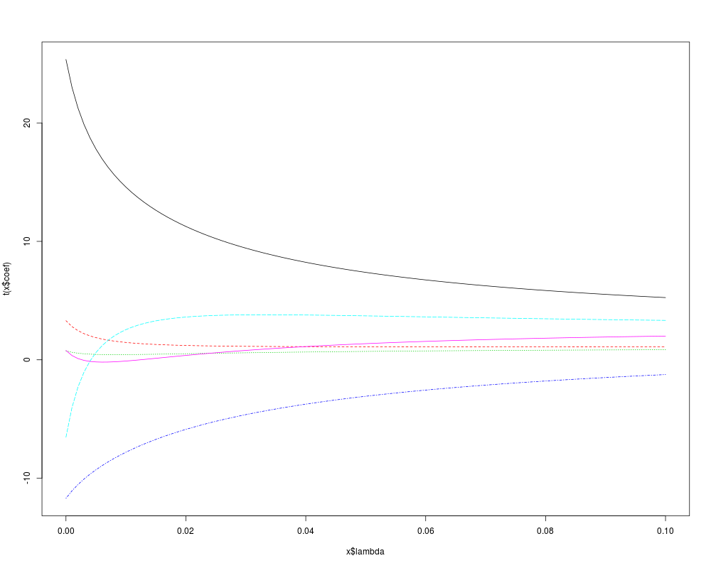
plot(lm.ridge(y ~ ., longley,
              lambda = seq(0,0.1,0.001)))
select(lm.ridge(y ~ ., longley,
               lambda = seq(0,0.1,0.0001)))

Results


R version 3.3.1 (2016-06-21) -- "Bug in Your Hair"
Copyright (C) 2016 The R Foundation for Statistical Computing
Platform: x86_64-pc-linux-gnu (64-bit)

R is free software and comes with ABSOLUTELY NO WARRANTY.
You are welcome to redistribute it under certain conditions.
Type 'license()' or 'licence()' for distribution details.

R is a collaborative project with many contributors.
Type 'contributors()' for more information and
'citation()' on how to cite R or R packages in publications.

Type 'demo()' for some demos, 'help()' for on-line help, or
'help.start()' for an HTML browser interface to help.
Type 'q()' to quit R.

> library(MASS)
> png(filename="/home/ddbj/snapshot/RGM3/R_CC/result/MASS/lm.ridge.Rd_%03d_medium.png", width=480, height=480)
> ### Name: lm.ridge
> ### Title: Ridge Regression
> ### Aliases: lm.ridge plot.ridgelm print.ridgelm select select.ridgelm
> ### Keywords: models
> 
> ### ** Examples
> 
> longley # not the same as the S-PLUS dataset
     GNP.deflator     GNP Unemployed Armed.Forces Population Year Employed
1947         83.0 234.289      235.6        159.0    107.608 1947   60.323
1948         88.5 259.426      232.5        145.6    108.632 1948   61.122
1949         88.2 258.054      368.2        161.6    109.773 1949   60.171
1950         89.5 284.599      335.1        165.0    110.929 1950   61.187
1951         96.2 328.975      209.9        309.9    112.075 1951   63.221
1952         98.1 346.999      193.2        359.4    113.270 1952   63.639
1953         99.0 365.385      187.0        354.7    115.094 1953   64.989
1954        100.0 363.112      357.8        335.0    116.219 1954   63.761
1955        101.2 397.469      290.4        304.8    117.388 1955   66.019
1956        104.6 419.180      282.2        285.7    118.734 1956   67.857
1957        108.4 442.769      293.6        279.8    120.445 1957   68.169
1958        110.8 444.546      468.1        263.7    121.950 1958   66.513
1959        112.6 482.704      381.3        255.2    123.366 1959   68.655
1960        114.2 502.601      393.1        251.4    125.368 1960   69.564
1961        115.7 518.173      480.6        257.2    127.852 1961   69.331
1962        116.9 554.894      400.7        282.7    130.081 1962   70.551
> names(longley)[1] <- "y"
> lm.ridge(y ~ ., longley)
                        GNP    Unemployed  Armed.Forces    Population 
2946.85636017    0.26352725    0.03648291    0.01116105   -1.73702984 
         Year      Employed 
  -1.41879853    0.23128785 
> plot(lm.ridge(y ~ ., longley,
+               lambda = seq(0,0.1,0.001)))
> select(lm.ridge(y ~ ., longley,
+                lambda = seq(0,0.1,0.0001)))
modified HKB estimator is 0.006836982 
modified L-W estimator is 0.05267247 
smallest value of GCV  at 0.0057 
> 
> 
> 
> 
> 
> dev.off()
null device 
          1 
>