R Graphical Manual

Browse All

Last data update: 2014.03.03

R: Ordered Logistic or Probit Regression

polr	R Documentation

Ordered Logistic or Probit Regression

Description

Fits a logistic or probit regression model to an ordered factor response. The default logistic case is proportional odds logistic regression, after which the function is named.

Usage

polr(formula, data, weights, start, ..., subset, na.action,
     contrasts = NULL, Hess = FALSE, model = TRUE,
     method = c("logistic", "probit", "loglog", "cloglog", "cauchit"))

Arguments

`formula`	a formula expression as for regression models, of the form `response ~ predictors`. The response should be a factor (preferably an ordered factor), which will be interpreted as an ordinal response, with levels ordered as in the factor. The model must have an intercept: attempts to remove one will lead to a warning and be ignored. An offset may be used. See the documentation of `formula` for other details.
`data`	an optional data frame in which to interpret the variables occurring in `formula`.
`weights`	optional case weights in fitting. Default to 1.
`start`	initial values for the parameters. This is in the format `c(coefficients, zeta)`: see the Values section.
`...`	additional arguments to be passed to `optim`, most often a `control` argument.
`subset`	expression saying which subset of the rows of the data should be used in the fit. All observations are included by default.
`na.action`	a function to filter missing data.
`contrasts`	a list of contrasts to be used for some or all of the factors appearing as variables in the model formula.
`Hess`	logical for whether the Hessian (the observed information matrix) should be returned. Use this if you intend to call `summary` or `vcov` on the fit.
`model`	logical for whether the model matrix should be returned.
`method`	logistic or probit or (complementary) log-log or cauchit (corresponding to a Cauchy latent variable).

Details

This model is what Agresti (2002) calls a cumulative link model. The basic interpretation is as a coarsened version of a latent variable Y_i which has a logistic or normal or extreme-value or Cauchy distribution with scale parameter one and a linear model for the mean. The ordered factor which is observed is which bin Y_i falls into with breakpoints

zeta_0 = -Inf < zeta_1 < … < zeta_K = Inf

This leads to the model

logit P(Y <= k | x) = zeta_k - eta

with logit replaced by probit for a normal latent variable, and eta being the linear predictor, a linear function of the explanatory variables (with no intercept). Note that it is quite common for other software to use the opposite sign for eta (and hence the coefficients beta).

In the logistic case, the left-hand side of the last display is the log odds of category k or less, and since these are log odds which differ only by a constant for different k, the odds are proportional. Hence the term proportional odds logistic regression.

The log-log and complementary log-log links are the increasing functions F^-1(p) = -log(-log(p)) and F^-1(p) = log(-log(1-p)); some call the first the ‘negative log-log’ link. These correspond to a latent variable with the extreme-value distribution for the maximum and minimum respectively.

A proportional hazards model for grouped survival times can be obtained by using the complementary log-log link with grouping ordered by increasing times.

predict, summary, vcov, anova, model.frame and an extractAIC method for use with stepAIC (and step). There are also profile and confint methods.

Value

A object of class "polr". This has components

`coefficients`	the coefficients of the linear predictor, which has no intercept.
`zeta`	the intercepts for the class boundaries.
`deviance`	the residual deviance.
`fitted.values`	a matrix, with a column for each level of the response.
`lev`	the names of the response levels.
`terms`	the `terms` structure describing the model.
`df.residual`	the number of residual degrees of freedoms, calculated using the weights.
`edf`	the (effective) number of degrees of freedom used by the model
`n, nobs`	the (effective) number of observations, calculated using the weights. (`nobs` is for use by `stepAIC`.
`call`	the matched call.
`method`	the matched method used.
`convergence`	the convergence code returned by `optim`.
`niter`	the number of function and gradient evaluations used by `optim`.
`lp`	the linear predictor (including any offset).
`Hessian`	(if `Hess` is true). Note that this is a numerical approximation derived from the optimization proces.
`model`	(if `model` is true).

Note

The vcov method uses the approximate Hessian: for reliable results the model matrix should be sensibly scaled with all columns having range the order of one.

Prior to version 7.3-32, method = "cloglog" confusingly gave the log-log link, implicitly assuming the first response level was the ‘best’.

References

Agresti, A. (2002) Categorical Data. Second edition. Wiley.

Venables, W. N. and Ripley, B. D. (2002) Modern Applied Statistics with S. Fourth edition. Springer.

Examples

options(contrasts = c("contr.treatment", "contr.poly"))
house.plr <- polr(Sat ~ Infl + Type + Cont, weights = Freq, data = housing)
house.plr
summary(house.plr, digits = 3)
## slightly worse fit from
summary(update(house.plr, method = "probit", Hess = TRUE), digits = 3)
## although it is not really appropriate, can fit
summary(update(house.plr, method = "loglog", Hess = TRUE), digits = 3)
summary(update(house.plr, method = "cloglog", Hess = TRUE), digits = 3)

predict(house.plr, housing, type = "p")
addterm(house.plr, ~.^2, test = "Chisq")
house.plr2 <- stepAIC(house.plr, ~.^2)
house.plr2$anova
anova(house.plr, house.plr2)

house.plr <- update(house.plr, Hess=TRUE)
pr <- profile(house.plr)
confint(pr)
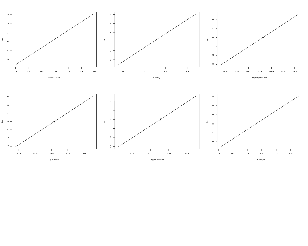
plot(pr)
pairs(pr)

Results


R version 3.3.1 (2016-06-21) -- "Bug in Your Hair"
Copyright (C) 2016 The R Foundation for Statistical Computing
Platform: x86_64-pc-linux-gnu (64-bit)

R is free software and comes with ABSOLUTELY NO WARRANTY.
You are welcome to redistribute it under certain conditions.
Type 'license()' or 'licence()' for distribution details.

R is a collaborative project with many contributors.
Type 'contributors()' for more information and
'citation()' on how to cite R or R packages in publications.

Type 'demo()' for some demos, 'help()' for on-line help, or
'help.start()' for an HTML browser interface to help.
Type 'q()' to quit R.

> library(MASS)
> png(filename="/home/ddbj/snapshot/RGM3/R_CC/result/MASS/polr.Rd_%03d_medium.png", width=480, height=480)
> ### Name: polr
> ### Title: Ordered Logistic or Probit Regression
> ### Aliases: polr
> ### Keywords: models
> 
> ### ** Examples
> 
> options(contrasts = c("contr.treatment", "contr.poly"))
> house.plr <- polr(Sat ~ Infl + Type + Cont, weights = Freq, data = housing)
> house.plr
Call:
polr(formula = Sat ~ Infl + Type + Cont, data = housing, weights = Freq)

Coefficients:
   InflMedium      InflHigh TypeApartment    TypeAtrium   TypeTerrace 
    0.5663937     1.2888191    -0.5723501    -0.3661866    -1.0910149 
     ContHigh 
    0.3602841 

Intercepts:
 Low|Medium Medium|High 
 -0.4961353   0.6907083 

Residual Deviance: 3479.149 
AIC: 3495.149 
> summary(house.plr, digits = 3)

Re-fitting to get Hessian

Call:
polr(formula = Sat ~ Infl + Type + Cont, data = housing, weights = Freq)

Coefficients:
               Value Std. Error t value
InflMedium     0.566     0.1047    5.41
InflHigh       1.289     0.1272   10.14
TypeApartment -0.572     0.1192   -4.80
TypeAtrium    -0.366     0.1552   -2.36
TypeTerrace   -1.091     0.1515   -7.20
ContHigh       0.360     0.0955    3.77

Intercepts:
            Value  Std. Error t value
Low|Medium  -0.496  0.125     -3.974 
Medium|High  0.691  0.125      5.505 

Residual Deviance: 3479.149 
AIC: 3495.149 
> ## slightly worse fit from
> summary(update(house.plr, method = "probit", Hess = TRUE), digits = 3)
Call:
polr(formula = Sat ~ Infl + Type + Cont, data = housing, weights = Freq, 
    Hess = TRUE, method = "probit")

Coefficients:
               Value Std. Error t value
InflMedium     0.346     0.0641    5.40
InflHigh       0.783     0.0764   10.24
TypeApartment -0.348     0.0723   -4.81
TypeAtrium    -0.218     0.0948   -2.30
TypeTerrace   -0.664     0.0918   -7.24
ContHigh       0.222     0.0581    3.83

Intercepts:
            Value  Std. Error t value
Low|Medium  -0.300  0.076     -3.937 
Medium|High  0.427  0.076      5.585 

Residual Deviance: 3479.689 
AIC: 3495.689 
> ## although it is not really appropriate, can fit
> summary(update(house.plr, method = "loglog", Hess = TRUE), digits = 3)
Call:
polr(formula = Sat ~ Infl + Type + Cont, data = housing, weights = Freq, 
    Hess = TRUE, method = "loglog")

Coefficients:
               Value Std. Error t value
InflMedium     0.367     0.0727    5.05
InflHigh       0.790     0.0806    9.81
TypeApartment -0.349     0.0757   -4.61
TypeAtrium    -0.196     0.0988   -1.98
TypeTerrace   -0.698     0.1043   -6.69
ContHigh       0.268     0.0636    4.21

Intercepts:
            Value  Std. Error t value
Low|Medium   0.086  0.083      1.038 
Medium|High  0.892  0.087     10.223 

Residual Deviance: 3491.41 
AIC: 3507.41 
> summary(update(house.plr, method = "cloglog", Hess = TRUE), digits = 3)
Call:
polr(formula = Sat ~ Infl + Type + Cont, data = housing, weights = Freq, 
    Hess = TRUE, method = "cloglog")

Coefficients:
               Value Std. Error t value
InflMedium     0.382     0.0703    5.44
InflHigh       0.915     0.0926    9.89
TypeApartment -0.407     0.0861   -4.73
TypeAtrium    -0.281     0.1111   -2.52
TypeTerrace   -0.742     0.1013   -7.33
ContHigh       0.209     0.0651    3.21

Intercepts:
            Value  Std. Error t value
Low|Medium  -0.796  0.090     -8.881 
Medium|High  0.055  0.086      0.647 

Residual Deviance: 3484.053 
AIC: 3500.053 
> 
> predict(house.plr, housing, type = "p")
         Low    Medium      High
1  0.3784493 0.2876752 0.3338755
2  0.3784493 0.2876752 0.3338755
3  0.3784493 0.2876752 0.3338755
4  0.2568264 0.2742122 0.4689613
5  0.2568264 0.2742122 0.4689613
6  0.2568264 0.2742122 0.4689613
7  0.1436924 0.2110836 0.6452240
8  0.1436924 0.2110836 0.6452240
9  0.1436924 0.2110836 0.6452240
10 0.5190445 0.2605077 0.2204478
11 0.5190445 0.2605077 0.2204478
12 0.5190445 0.2605077 0.2204478
13 0.3798514 0.2875965 0.3325521
14 0.3798514 0.2875965 0.3325521
15 0.3798514 0.2875965 0.3325521
16 0.2292406 0.2643196 0.5064398
17 0.2292406 0.2643196 0.5064398
18 0.2292406 0.2643196 0.5064398
19 0.4675584 0.2745383 0.2579033
20 0.4675584 0.2745383 0.2579033
21 0.4675584 0.2745383 0.2579033
22 0.3326236 0.2876008 0.3797755
23 0.3326236 0.2876008 0.3797755
24 0.3326236 0.2876008 0.3797755
25 0.1948548 0.2474226 0.5577225
26 0.1948548 0.2474226 0.5577225
27 0.1948548 0.2474226 0.5577225
28 0.6444840 0.2114256 0.1440905
29 0.6444840 0.2114256 0.1440905
30 0.6444840 0.2114256 0.1440905
31 0.5071210 0.2641196 0.2287594
32 0.5071210 0.2641196 0.2287594
33 0.5071210 0.2641196 0.2287594
34 0.3331573 0.2876330 0.3792097
35 0.3331573 0.2876330 0.3792097
36 0.3331573 0.2876330 0.3792097
37 0.2980880 0.2837746 0.4181374
38 0.2980880 0.2837746 0.4181374
39 0.2980880 0.2837746 0.4181374
40 0.1942209 0.2470589 0.5587202
41 0.1942209 0.2470589 0.5587202
42 0.1942209 0.2470589 0.5587202
43 0.1047770 0.1724227 0.7228003
44 0.1047770 0.1724227 0.7228003
45 0.1047770 0.1724227 0.7228003
46 0.4294564 0.2820629 0.2884807
47 0.4294564 0.2820629 0.2884807
48 0.4294564 0.2820629 0.2884807
49 0.2993357 0.2839753 0.4166890
50 0.2993357 0.2839753 0.4166890
51 0.2993357 0.2839753 0.4166890
52 0.1718050 0.2328648 0.5953302
53 0.1718050 0.2328648 0.5953302
54 0.1718050 0.2328648 0.5953302
55 0.3798387 0.2875972 0.3325641
56 0.3798387 0.2875972 0.3325641
57 0.3798387 0.2875972 0.3325641
58 0.2579546 0.2745537 0.4674917
59 0.2579546 0.2745537 0.4674917
60 0.2579546 0.2745537 0.4674917
61 0.1444202 0.2117081 0.6438717
62 0.1444202 0.2117081 0.6438717
63 0.1444202 0.2117081 0.6438717
64 0.5583813 0.2471826 0.1944361
65 0.5583813 0.2471826 0.1944361
66 0.5583813 0.2471826 0.1944361
67 0.4178031 0.2838213 0.2983756
68 0.4178031 0.2838213 0.2983756
69 0.4178031 0.2838213 0.2983756
70 0.2584149 0.2746916 0.4668935
71 0.2584149 0.2746916 0.4668935
72 0.2584149 0.2746916 0.4668935
> addterm(house.plr, ~.^2, test = "Chisq")
Single term additions

Model:
Sat ~ Infl + Type + Cont
          Df    AIC     LRT   Pr(Chi)    
<none>       3495.1                      
Infl:Type  6 3484.6 22.5093 0.0009786 ***
Infl:Cont  2 3498.9  0.2090 0.9007957    
Type:Cont  3 3492.5  8.6662 0.0340752 *  
---
Signif. codes:  0 '***' 0.001 '**' 0.01 '*' 0.05 '.' 0.1 ' ' 1
> house.plr2 <- stepAIC(house.plr, ~.^2)
Start:  AIC=3495.15
Sat ~ Infl + Type + Cont

            Df    AIC
+ Infl:Type  6 3484.6
+ Type:Cont  3 3492.5
<none>         3495.1
+ Infl:Cont  2 3498.9
- Cont       1 3507.5
- Type       3 3545.1
- Infl       2 3599.4

Step:  AIC=3484.64
Sat ~ Infl + Type + Cont + Infl:Type

            Df    AIC
+ Type:Cont  3 3482.7
<none>         3484.6
+ Infl:Cont  2 3488.5
- Infl:Type  6 3495.1
- Cont       1 3497.8

Step:  AIC=3482.69
Sat ~ Infl + Type + Cont + Infl:Type + Type:Cont

            Df    AIC
<none>         3482.7
- Type:Cont  3 3484.6
+ Infl:Cont  2 3486.6
- Infl:Type  6 3492.5
> house.plr2$anova
Stepwise Model Path 
Analysis of Deviance Table

Initial Model:
Sat ~ Infl + Type + Cont

Final Model:
Sat ~ Infl + Type + Cont + Infl:Type + Type:Cont


         Step Df  Deviance Resid. Df Resid. Dev      AIC
1                               1673   3479.149 3495.149
2 + Infl:Type  6 22.509347      1667   3456.640 3484.640
3 + Type:Cont  3  7.945029      1664   3448.695 3482.695
> anova(house.plr, house.plr2)
Likelihood ratio tests of ordinal regression models

Response: Sat
                                       Model Resid. df Resid. Dev   Test    Df
1                         Infl + Type + Cont      1673   3479.149             
2 Infl + Type + Cont + Infl:Type + Type:Cont      1664   3448.695 1 vs 2     9
  LR stat.      Pr(Chi)
1                      
2 30.45438 0.0003670555
> 
> house.plr <- update(house.plr, Hess=TRUE)
> pr <- profile(house.plr)
> confint(pr)
                   2.5 %      97.5 %
InflMedium     0.3616415  0.77195375
InflHigh       1.0409701  1.53958138
TypeApartment -0.8069590 -0.33940432
TypeAtrium    -0.6705862 -0.06204495
TypeTerrace   -1.3893863 -0.79533958
ContHigh       0.1733589  0.54792854
> plot(pr)
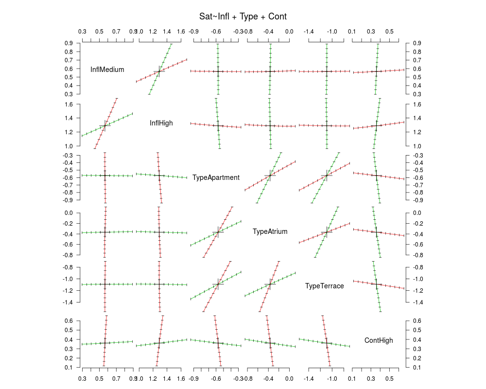
> pairs(pr)
> 
> 
> 
> 
> 
> dev.off()
null device 
          1 
>