R Graphical Manual

Browse All

Last data update: 2014.03.03

R: Regression Surface Containing Interaction

intr.plot

R Documentation

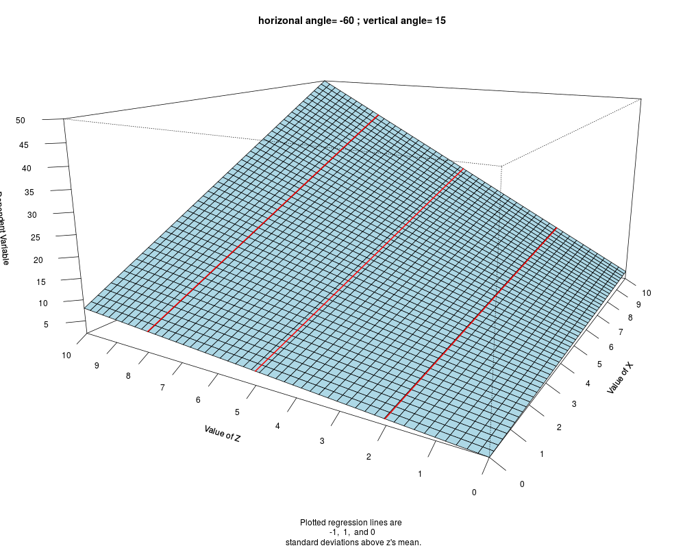
Regression Surface Containing Interaction

Description

To plot a three dimentional figure of a multiple regression surface containing one two-way interaction.

Usage

intr.plot(b.0, b.x, b.z, b.xz, x.min = NULL, x.max = NULL, z.min = NULL, 
z.max = NULL, n.x = 50, n.z = 50, x = NULL, z = NULL, col = "lightblue", 
hor.angle = -60, vert.angle = 15, xlab = "Value of X", zlab = "Value of Z", 
ylab = "Dependent Variable", expand = 0.5, lines.plot=TRUE, col.line = "red", 
line.wd = 2, gray.scale = FALSE, ticktype="detailed", ...)

Arguments

`b.0`	the intercept
`b.x`	regression coefficient for predictor x
`b.z`	regression coefficient for predictor z
`b.xz`	regression coefficient for the interaction of predictors x and z
`x.min, x.max, z.min, z.max`	ranges of x and z. The regression surface defined by these limits will be plotted.
`n.x`	number of elements in predictor vector x; number of points to be plotted on the regression surface; default is 50
`n.z`	number of elements in predictor vector z; number of points to be plotted on the regression surface; default is 50
`x`	a specific predictor vector x, used instead of `x.max` and `x.min`
`z`	a specific predictor vector z, used instead of `z.max` and `z.min`
`col`	color of the regression surface; default is `"lightbule"`
`hor.angle`	rotate the regression surface horizontally; default is -60 degree
`vert.angle`	rotate the regression surface vertically; default is 15 degree
`xlab`	title for the axis which the predictor x is on
`zlab`	title for the axis which the predictor z is on
`ylab`	title for the axis which the dependent y is on
`expand`	default is 0.5; expansion factor applied to the axis of the dependent variable. Often used with 0 < `expand` < 1 to shrink the plotting box in the direction of the dependent variable's axis.
`lines.plot`	whether or not to plot on the regression surface regression lines holding z at values 0, 1, -1, 2, -2 above the mean; default is TRUE.
`col.line`	the color of regression lines plotted on the regression surface; default is red
`line.wd`	the width of regression lines plotted on the regression surface; default is 2
`gray.scale`	whether or not to plot the figure black and white; default is FALSE
`ticktype`	whether the axes should be plotted with (`"detailed"`) or without (`"simple"`) tick marks
`...`	allows one to potentially include parameter values for inner functions

Details

The user can input either the limits of x and z, or specific x and z vectors, to draw the regression surface. If the user inputs simply the limits of the predictors, the function would generate predictor vectors for plotting. If the user inputs specific predictor vectors, the function would plot the regression surface based on those vectors.

Note

If the user enters specific vectors instead of the ranges of predictors, please make sure elements in those vectors are in ascending order. This is required by function persp, which is used within this function.

Author(s)

Keke Lai (University of California – Merced; klai25@ucmerced.edu) and Ken Kelley (University of Notre Dame; KKelley@ND.Edu)

References

Cohen, J., Cohen, P., West, S. G. and Aiken, L. S. (2003). Applied multiple regression/correlation analysis for the behavioral sciences (3rd ed.). Mahwah, NJ: Erlbaum.

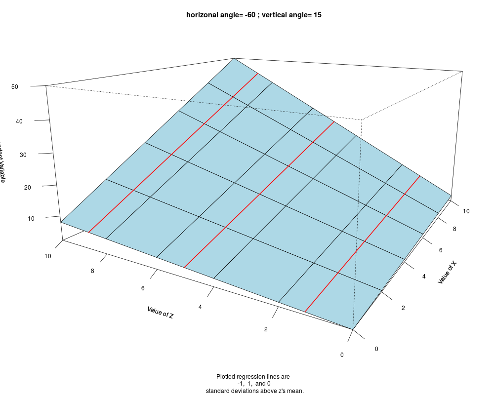
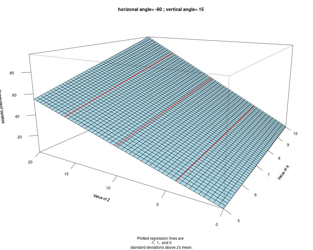
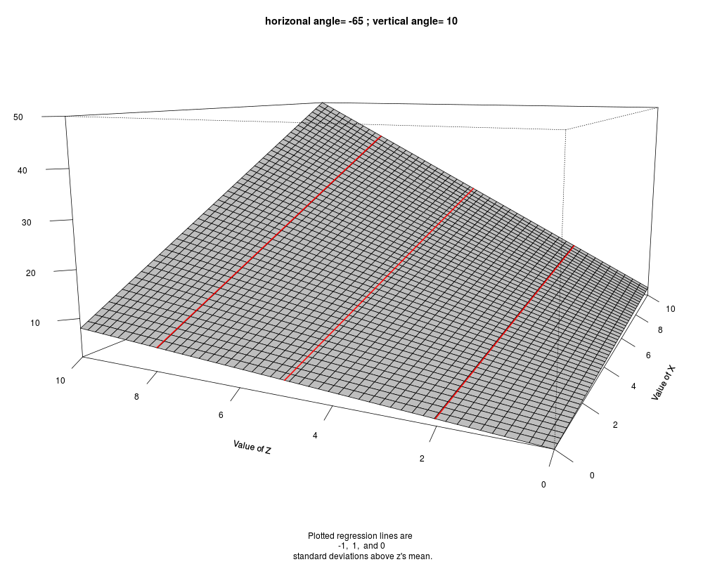
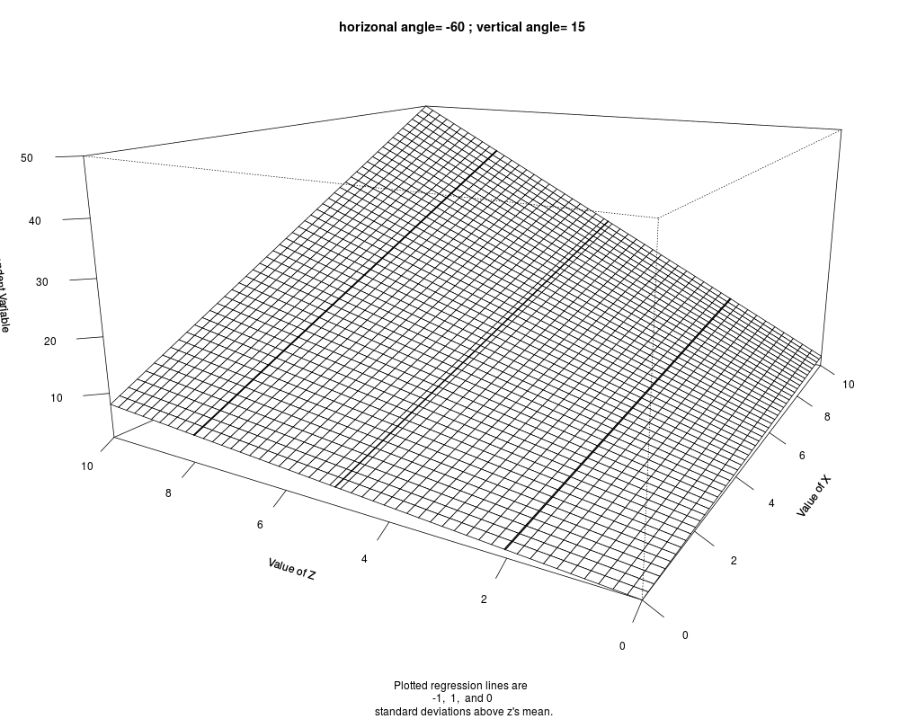
Examples

##  A way to replicate the example given by Cohen et al. (2003) (pp. 258--263):
##  The regression equation with interaction is y=.2X+.6Z+.4XZ+2
##  To plot a regression surface and regression lines of Y on X holding Z 
##  at -1, 0, and 1 standard deviation above the mean

x<- c(0,2,4,6,8,10)
z<-c(0,2,4,6,8,10)
intr.plot(b.0=2, b.x=.2, b.z=.6, b.xz=.4, x=x, z=z)

## input limits of the predictors instead of specific x and z predictor vectors
intr.plot(b.0=2, b.x=.2, b.z=.6, b.xz=.4, x.min=5, x.max=10, z.min=0, z.max=20)

intr.plot(b.0=2, b.x=.2, b.z=.6, b.xz=.4, x.min=0, x.max=10, z.min=0, z.max=10, 
col="gray", hor.angle=-65, vert.angle=10)

##  To plot a black-and-white figure
intr.plot(b.0=2, b.x=.2, b.z=.6, b.xz=.4, x.min=0, x.max=10, z.min=0, z.max=10, 
gray.scale=TRUE)

## to adjust the tick marks on the axes
intr.plot(b.0=2, b.x=.2, b.z=.6, b.xz=.4, x.min=0, x.max=10, z.min=0, z.max=10, 
ticktype="detailed", nticks=8)

Results


R version 3.3.1 (2016-06-21) -- "Bug in Your Hair"
Copyright (C) 2016 The R Foundation for Statistical Computing
Platform: x86_64-pc-linux-gnu (64-bit)

R is free software and comes with ABSOLUTELY NO WARRANTY.
You are welcome to redistribute it under certain conditions.
Type 'license()' or 'licence()' for distribution details.

R is a collaborative project with many contributors.
Type 'contributors()' for more information and
'citation()' on how to cite R or R packages in publications.

Type 'demo()' for some demos, 'help()' for on-line help, or
'help.start()' for an HTML browser interface to help.
Type 'q()' to quit R.

> library(MBESS)
> png(filename="/home/ddbj/snapshot/RGM3/R_CC/result/MBESS/intr.plot.Rd_%03d_medium.png", width=480, height=480)
> ### Name: intr.plot
> ### Title: Regression Surface Containing Interaction
> ### Aliases: intr.plot
> ### Keywords: regression
> 
> ### ** Examples
> 
> ##  A way to replicate the example given by Cohen et al. (2003) (pp. 258--263):
> ##  The regression equation with interaction is y=.2X+.6Z+.4XZ+2
> ##  To plot a regression surface and regression lines of Y on X holding Z 
> ##  at -1, 0, and 1 standard deviation above the mean
> 
> x<- c(0,2,4,6,8,10)
> z<-c(0,2,4,6,8,10)
> intr.plot(b.0=2, b.x=.2, b.z=.6, b.xz=.4, x=x, z=z)
> 
> ## input limits of the predictors instead of specific x and z predictor vectors
> intr.plot(b.0=2, b.x=.2, b.z=.6, b.xz=.4, x.min=5, x.max=10, z.min=0, z.max=20)
> 
> intr.plot(b.0=2, b.x=.2, b.z=.6, b.xz=.4, x.min=0, x.max=10, z.min=0, z.max=10, 
+ col="gray", hor.angle=-65, vert.angle=10)
> 
> ##  To plot a black-and-white figure
> intr.plot(b.0=2, b.x=.2, b.z=.6, b.xz=.4, x.min=0, x.max=10, z.min=0, z.max=10, 
+ gray.scale=TRUE)
> 
> ## to adjust the tick marks on the axes
> intr.plot(b.0=2, b.x=.2, b.z=.6, b.xz=.4, x.min=0, x.max=10, z.min=0, z.max=10, 
+ ticktype="detailed", nticks=8)
> 
> 
> 
> 
> 
> dev.off()
null device 
          1 
>