R Graphical Manual

Browse All

Last data update: 2014.03.03

R: Calculation of the melting temperature (Tm) from the first...

diffQ

R Documentation

Calculation of the melting temperature (Tm) from the first derivative

Description

diffQ is used to calculate the melting temperature (Tm) but also for elementary graphical operations (e.g., show the Tm or the derivative). It does not require smoothed data for the MCA. The parameter rsm can be used to double the temperature resolution by calculation of the mean temperature and mean fluorescence. Note: mcaSmoother has the n parameter with a similar functionality. First the approximate Tm is determined as the min() and/or max() from the first derivative. The first numeric derivative (Forward Difference) is estimated from the values of the function values obtained during an experiment since the exact function of the melting curve is unknown. The method used in diffQ is suitable for independent variables that are equally and unequally spaced. Alternatives for the numerical differentiation include Backward Differences, Central Differences or Three-Point (Forward or Backward) Difference based on Lagrange Estimation (currently not implemented in diffQ). The approximate peak value is the starting-point for a function based calculation. The function takes a defined number n (maximum 8) of the left and the right neighbor values and fits a quadratic polynomial. The quadratic regression of the X (temperature) against the Y (fluorescence) range gives the coefficients. The optimal quadratic polynomial is chosen based on the highest adjusted R-squared value. diffQ returns an objects of the class list. To accessing components of lists is done as described elsewhere either by name or by number. diffQ has a simple plot function. However, for sophisticated analysis and plots its recommended to use diffQ as presented in the examples as part of algorithms.

Usage

diffQ(xy, fct = min, fws = 8, col = 2, plot = FALSE, verbose = FALSE,
  warn = TRUE, peak = FALSE, negderiv = TRUE, deriv = FALSE,
  derivlimits = FALSE, derivlimitsline = FALSE, vertiline = FALSE,
  rsm = FALSE, inder = FALSE)

Arguments

`xy`	is a `data.frame` containing in the first column the temperature and in the second column the fluorescence values. Preferably the output from `mcaSmoother` is used.
`fct`	accepts `min` or `max` as option and is used to define whether to find a local minimum (“negative peak”) or local maximum (“positive peak”).
`fws`	defines the number (n) of left and right neighbors to use for the calculation of the quadratic polynomial.
`col`	is a graphical parameter used to define the length of the line used in the plot.
`plot`	shows a plot of a single melting curve. To draw multiple curves in a single plot set `plot = FALSE` and create and empty plot instead (see examples).
`verbose`	shows additional information (e.g., approximate derivative, ranges used for calculation, approximate Tm) of the calculation.
`warn`	diffQ tries to keep the user as informed as possible about the quality of the analysis. However, in some scenarios are the warning and message about analysis not needed or disturbing. `warn` can be used to stop the flodding of the output.
`peak`	shows the peak in the plot (see examples).
`negderiv`	uses the positive first derivative instead of the negative.
`deriv`	shows the first derivative with the color assigned to `col` (see examples).
`derivlimits`	shows the neighbors (fws) used to calculate the Tm as points in the plot (see examples).
`derivlimitsline`	shows the neighbors (fws) used to calculate the Tm as line in the plot (see examples).
`vertiline`	draws a vertical line at the Tms (see examples).
`rsm`	performs a doubling of the temperature resolution by calculation of the mean temperature and mean fluorescence between successive temperature steps. Note: `mcaSmoother` has the "n" parameter with a similar but advanced functionality.
`inder`	Interpolates first derivatives using the five-point stencil. See `chipPCR` package for details.

Value

`diffQ()`	returns a comprehensive list (if parameter verbose is TRUE) with results from the first derivative. The list includes a `data.frame` of the derivative ("xy"). The temperature range ("limits.xQ") and fluorescence range ("limits.diffQ") to calculate the peak value. "fluo.x" is the approximate fluorescence at the approximate melting temperature. The calculated melting temperature ("Tm") with the corresponding fluorescence intensity ("fluoTm"). The number of neighbors ("fws"), the adjusted R-squared ("adj.r.squared") and the normalized-root-mean-squared-error ("NRMSE") to fit. The quality of the calculated melting temperature ("Tm") can be checked with devsum which reports the relative deviation (in percent) between the approximate melting temperature and the calculated melting temperature, if NRMSE is less than 0.08 and the adjusted R-squared is less than 0.85. A relative deviation larger than 10 percent will result in a warning. Reducing fws might improve the result.
`Tm`	returns the calculated melting temperature ("Tm").
`fluoTm`	returns the calculated fluorescence at the calculated melting temperature.
`Tm.approx`	returns the approximate melting temperature.
`fluo.x`	returns the approximate fluorescence at the calculated melting temperature.
`xy`	returns the approximate derivative value used for the calculation of the melting peak.
`limits.xQ`	returns a data range of temperature values used to calculate the melting temperature.
`limits.diffQ`	returns a data range of fluorescence values used to calculate the melting temperature.
`adj.r.squared`	returns the adjusted R-squared from the quadratic model fitting function (see also `fit`).
`NRMSE`	returns the normalized root-mean-squared-error (NRMSE) from the quadratic model fitting function (see also `fit`).
`fws`	returns the number of points used for the calculation of the melting temperature.
`devsum`	returns measures to show the difference between the approximate and calculated melting temperature.
`temperature`	returns measures to investigate the temperature resolution of the melting curve. Raw fluorescence measurements at irregular temperature resolutions (intervals) can introduce artifacts and thus lead to wrong melting point estimations.
`temperature$T.delta`	returns the difference between two successive temperature steps.
`temperature$mean.T.delta`	returns the mean difference between two temperature steps.
`temperature$sd.T.delta`	returns the standard deviation of the temperature.
`temperature$RSD.T.delta`	returns the relative standard deviation (RSD) of the temperature in percent.
`fit`	returns the summary of the results of the quadratic model fitting function.

Author(s)

Stefan Roediger

References

A Highly Versatile Microscope Imaging Technology Platform for the Multiplex Real-Time Detection of Biomolecules and Autoimmune Antibodies. S. Roediger, P. Schierack, A. Boehm, J. Nitschke, I. Berger, U. Froemmel, C. Schmidt, M. Ruhland, I. Schimke, D. Roggenbuck, W. Lehmann and C. Schroeder. Advances in Biochemical Bioengineering/Biotechnology. 133:33–74, 2013. http://www.ncbi.nlm.nih.gov/pubmed/22437246

Nucleic acid detection based on the use of microbeads: a review. S. Roediger, C. Liebsch, C. Schmidt, W. Lehmann, U. Resch-Genger, U. Schedler, P. Schierack. Microchim Acta 2014:1–18. DOI: 10.1007/s00604-014-1243-4

Roediger S, Boehm A, Schimke I. Surface Melting Curve Analysis with R. The R Journal 2013;5:37–53.

Examples

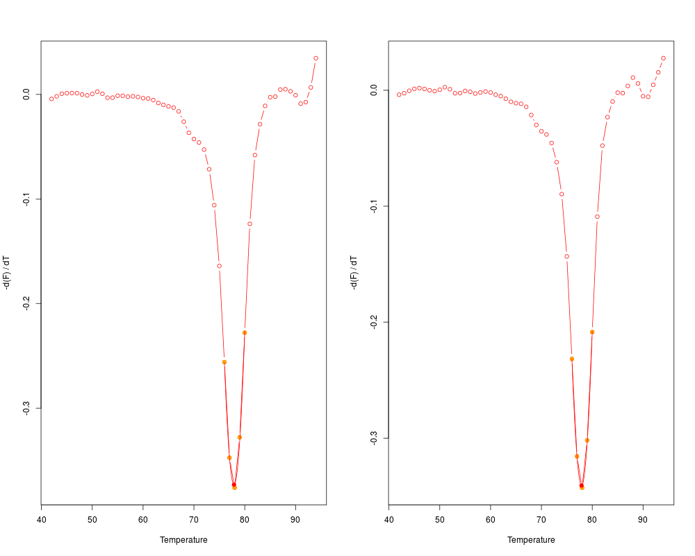
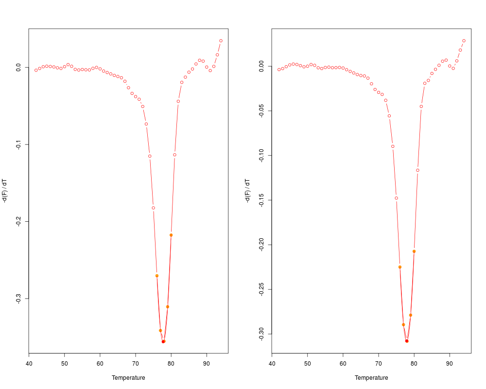
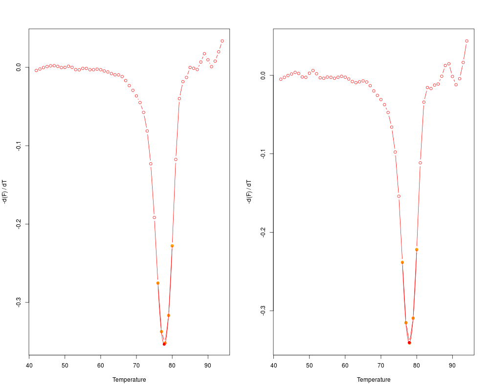
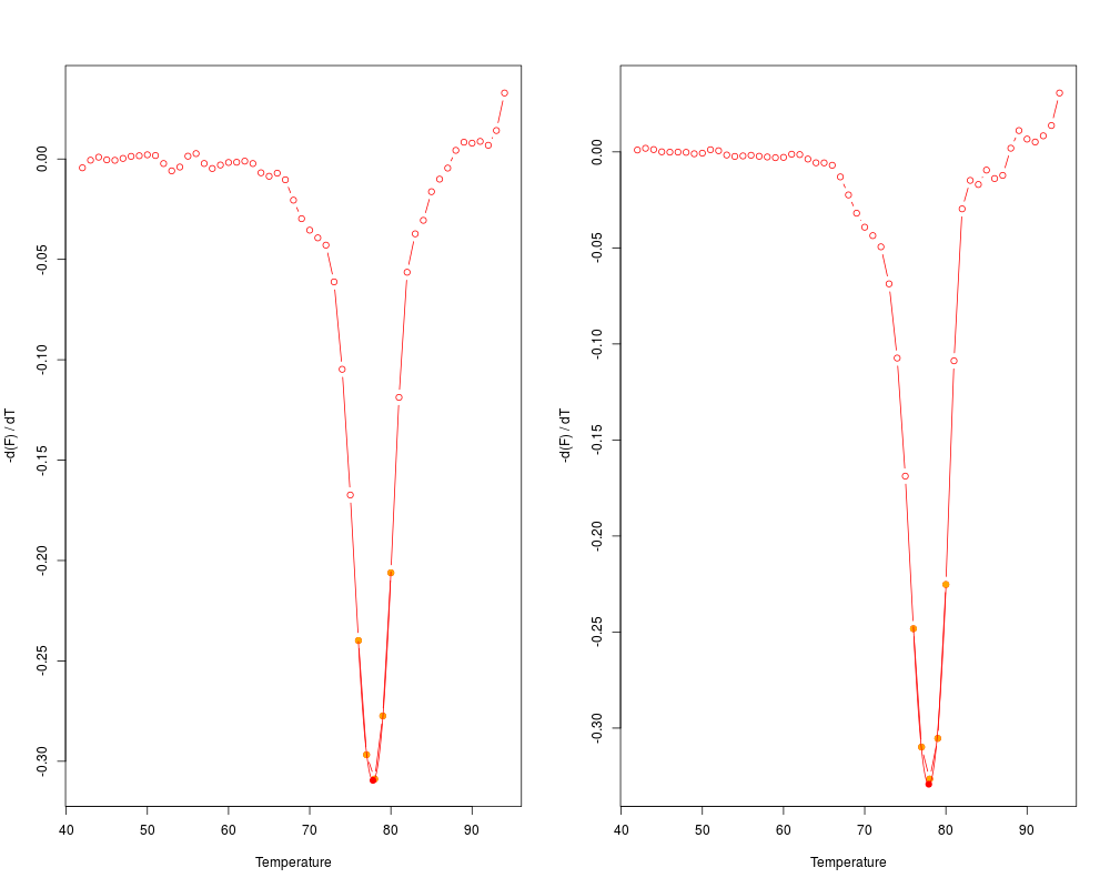
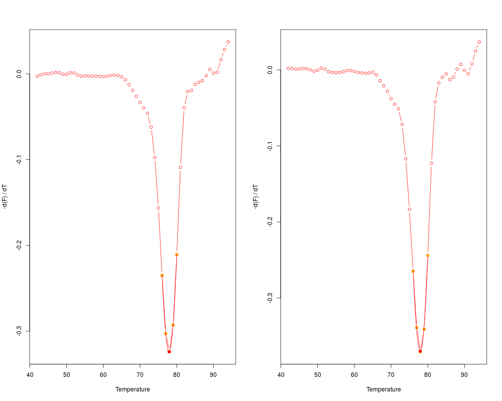
# First Example
# Plot the first derivative of different samples for single melting curve
# data. Note that the argument "plot" is TRUE.

data(MultiMelt)
par(mfrow = c(1,2))
sapply(2L:14, function(i) {
        tmp <- mcaSmoother(MultiMelt[, 1], MultiMelt[, i])
        diffQ(tmp, plot = TRUE)
  }
)
par(mfrow = c(1,1))
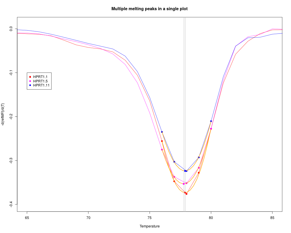
# Second example
# Plot the first derivative of different samples from MultiMelt
# in a single plot.
data(MultiMelt)

# First create an empty plot
plot(NA, NA, xlab = "Temperature", ylab ="-d(refMFI)/d(T)",
        main = "Multiple melting peaks in a single plot", xlim = c(65,85),
        ylim = c(-0.4,0.01), pch = 19, cex = 1.8)
# Prepossess the selected melting curve data (2,6,12) with mcaSmoother
# and apply them to diffQ. Note that the argument "plot" is FALSE
# while other arguments like derivlimitsline or peak are TRUE.
sapply(c(2,6,12), function(i) {
	tmp <- mcaSmoother(MultiMelt[, 1], MultiMelt[, i],
			    bg = c(41,61), bgadj = TRUE)
	diffQ(tmp, plot = FALSE, derivlimitsline = TRUE, deriv = TRUE,
	      peak = TRUE, derivlimits = TRUE, col = i, vertiline = TRUE)
  }
)
legend(65, -0.1, colnames(MultiMelt[, c(2,6,12)]), pch = c(15,15,15),
	col = c(2,6,12))

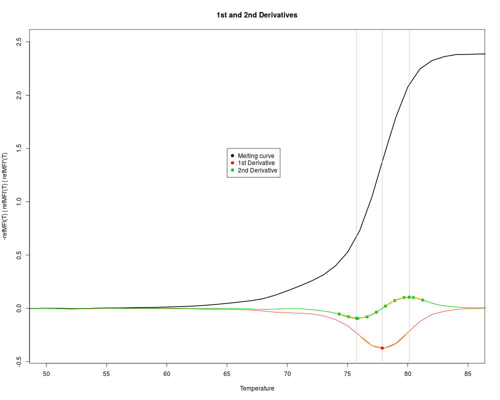
# Third example
# First create an empty plot
plot(NA, NA, xlim = c(50,85), ylim = c(-0.4,2.5),
     xlab = "Temperature",
     ylab ="-refMFI(T) | refMFI'(T) | refMFI''(T)",
     main = "1st and 2nd Derivatives",
     pch = 19, cex = 1.8)

# Prepossess the selected melting curve data with mcaSmoother
# and apply them to diffQ and diffQ2. Note that
# the argument "plot" is FALSE while other
# arguments like derivlimitsline or peak are TRUE.

tmp <- mcaSmoother(MultiMelt[, 1], MultiMelt[, 2],
		    bg = c(41,61), bgadj = TRUE)
lines(tmp, col= 1, lwd = 2)

# Note the different use of the argument derivlimits in diffQ and diffQ2
diffQ(tmp, fct = min, derivlimitsline = TRUE, deriv = TRUE,
	    peak = TRUE, derivlimits = FALSE, col = 2, vertiline = TRUE)
diffQ2(tmp, fct = min, derivlimitsline = TRUE, deriv = TRUE,
	    peak = TRUE, derivlimits = TRUE, col = 3, vertiline = TRUE)

# Add a legend to the plot
legend(65, 1.5, c("Melting curve",
		  "1st Derivative",
		  "2nd Derivative"),
		  pch = c(19,19,19), col = c(1,2,3))

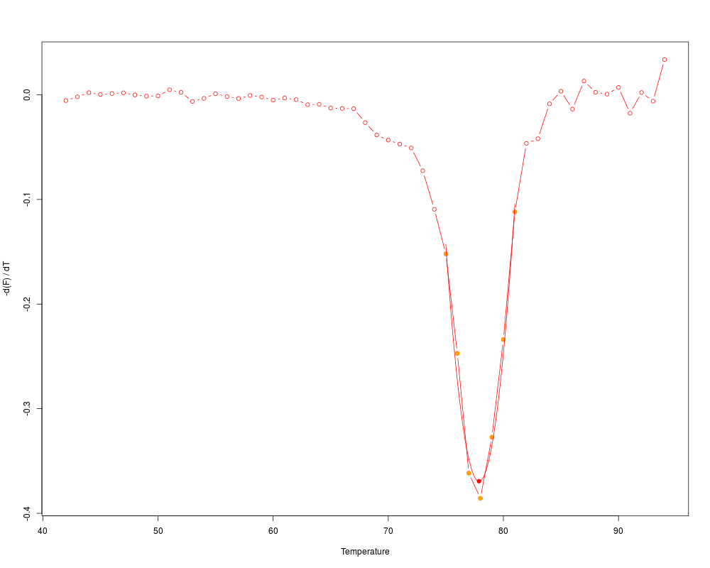
# Fourth example
# Different curves may potentially have different quality in practice.
# For example, using data from MultiMelt should return a
# valid result and plot.
data(MultiMelt)

diffQ(cbind(MultiMelt[, 1], MultiMelt[, 2]), plot = TRUE)$Tm
# limits_xQ
#  77.88139

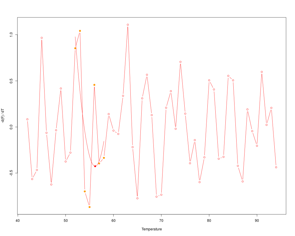
# Imagine an experiment that went terribly wrong. You would
# still get an estimate for the Tm. The output from diffQ,
# with an error attached, lets the user know that this Tm
# is potentially meaningless. diffQ() will give several
# warning messages.

set.seed(1)
y = rnorm(55,1.5,.8)
diffQ(cbind(MultiMelt[, 1],y), plot = TRUE)$Tm

# The distribution of the curve data indicates noise.
# The data should be visually inspected with a plot
# (see examples of diffQ). The Tm calculation (fit,
# adj. R squared ~ 0.157, NRMSE ~ 0.279) is not optimal
# presumably due to noisy data. Check raw melting
# curve (see examples of diffQ).
# Calculated Tm
#      56.16755


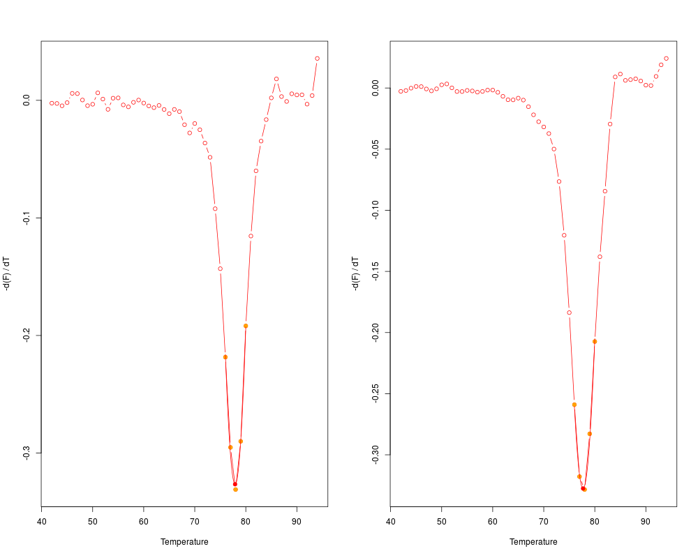
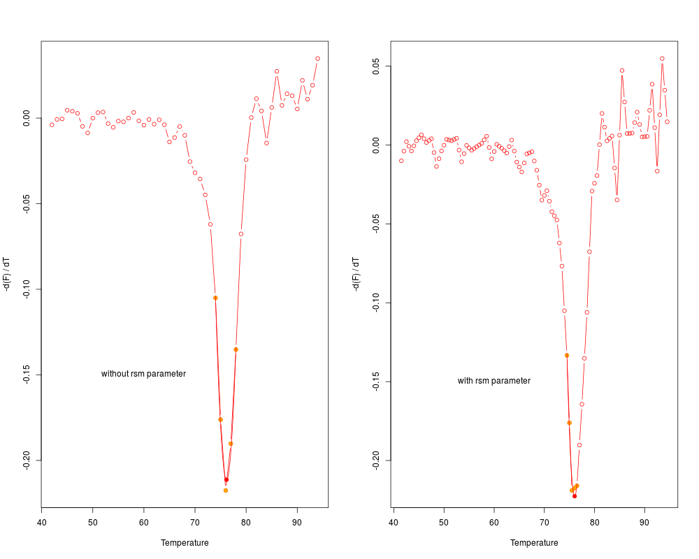
# Sixth example
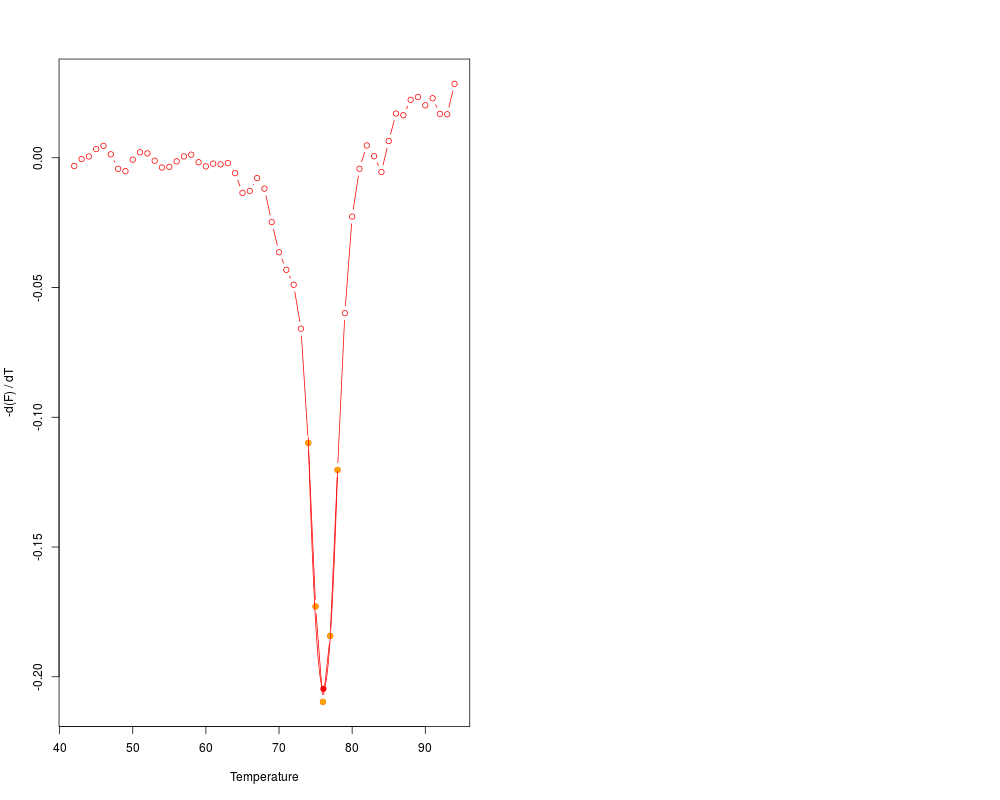
# Curves may potentially have a low temperature resolution. The rsm
# parameter can be used to double the temperature resolution.
# Use data from MultiMelt column 15 (MLC2v2).
data(MultiMelt)
tmp <- cbind(MultiMelt[, 1], MultiMelt[, 15])

# Use diffQ without and with the rsm parameter and plot
# the results in a single row
par(mfrow = c(1,2))

diffQ(tmp, plot = TRUE)$Tm
  text(60, -0.15, "without rsm parameter")

diffQ(tmp, plot = TRUE, rsm = TRUE)$Tm
  text(60, -0.15, "with rsm parameter")
par(mfrow = c(1,1))

Results


R version 3.3.1 (2016-06-21) -- "Bug in Your Hair"
Copyright (C) 2016 The R Foundation for Statistical Computing
Platform: x86_64-pc-linux-gnu (64-bit)

R is free software and comes with ABSOLUTELY NO WARRANTY.
You are welcome to redistribute it under certain conditions.
Type 'license()' or 'licence()' for distribution details.

R is a collaborative project with many contributors.
Type 'contributors()' for more information and
'citation()' on how to cite R or R packages in publications.

Type 'demo()' for some demos, 'help()' for on-line help, or
'help.start()' for an HTML browser interface to help.
Type 'q()' to quit R.

> library(MBmca)
Loading required package: robustbase
Loading required package: chipPCR
> png(filename="/home/ddbj/snapshot/RGM3/R_CC/result/MBmca/diffQ.Rd_%03d_medium.png", width=480, height=480)
> ### Name: diffQ
> ### Title: Calculation of the melting temperature (Tm) from the first
> ###   derivative
> ### Aliases: diffQ
> ### Keywords: Tm melting
> 
> ### ** Examples
> 
> # First Example
> # Plot the first derivative of different samples for single melting curve
> # data. Note that the argument "plot" is TRUE.
> 
> data(MultiMelt)
> par(mfrow = c(1,2))
> sapply(2L:14, function(i) {
+         tmp <- mcaSmoother(MultiMelt[, 1], MultiMelt[, i])
+         diffQ(tmp, plot = TRUE)
+   }
+ )
       [,1]       [,2]       [,3]       [,4]       [,5]       [,6]      
Tm     77.88494   77.90029   77.75343   77.89949   77.76936   77.93054  
fluoTm -0.3732338 -0.3408576 -0.3560144 -0.3076871 -0.3532675 -0.3405116
       [,7]       [,8]       [,9]       [,10]      [,11]      [,12]    
Tm     77.90438   77.7017    77.79736   77.88993   77.8833    77.93199 
fluoTm -0.3265402 -0.3275499 -0.3095232 -0.3292306 -0.3237404 -0.369646
       [,13]     
Tm     76.07117  
fluoTm -0.2046684
> par(mfrow = c(1,1))
> # Second example
> # Plot the first derivative of different samples from MultiMelt
> # in a single plot.
> data(MultiMelt)
> 
> # First create an empty plot
> plot(NA, NA, xlab = "Temperature", ylab ="-d(refMFI)/d(T)",
+         main = "Multiple melting peaks in a single plot", xlim = c(65,85),
+         ylim = c(-0.4,0.01), pch = 19, cex = 1.8)
> # Prepossess the selected melting curve data (2,6,12) with mcaSmoother
> # and apply them to diffQ. Note that the argument "plot" is FALSE
> # while other arguments like derivlimitsline or peak are TRUE.
> sapply(c(2,6,12), function(i) {
+ 	tmp <- mcaSmoother(MultiMelt[, 1], MultiMelt[, i],
+ 			    bg = c(41,61), bgadj = TRUE)
+ 	diffQ(tmp, plot = FALSE, derivlimitsline = TRUE, deriv = TRUE,
+ 	      peak = TRUE, derivlimits = TRUE, col = i, vertiline = TRUE)
+   }
+ )
       [,1]       [,2]       [,3]      
Tm     77.88494   77.76936   77.8833   
fluoTm -0.3731492 -0.3532051 -0.3237496
> legend(65, -0.1, colnames(MultiMelt[, c(2,6,12)]), pch = c(15,15,15),
+ 	col = c(2,6,12))
> 
> # Third example
> # First create an empty plot
> plot(NA, NA, xlim = c(50,85), ylim = c(-0.4,2.5),
+      xlab = "Temperature",
+      ylab ="-refMFI(T) | refMFI'(T) | refMFI''(T)",
+      main = "1st and 2nd Derivatives",
+      pch = 19, cex = 1.8)
> 
> # Prepossess the selected melting curve data with mcaSmoother
> # and apply them to diffQ and diffQ2. Note that
> # the argument "plot" is FALSE while other
> # arguments like derivlimitsline or peak are TRUE.
> 
> tmp <- mcaSmoother(MultiMelt[, 1], MultiMelt[, 2],
+ 		    bg = c(41,61), bgadj = TRUE)
> lines(tmp, col= 1, lwd = 2)
> 
> # Note the different use of the argument derivlimits in diffQ and diffQ2
> diffQ(tmp, fct = min, derivlimitsline = TRUE, deriv = TRUE,
+ 	    peak = TRUE, derivlimits = FALSE, col = 2, vertiline = TRUE)
Calculated Tm: 77.88494 
Signal height at calculated Tm: -0.3731492 
> diffQ2(tmp, fct = min, derivlimitsline = TRUE, deriv = TRUE,
+ 	    peak = TRUE, derivlimits = TRUE, col = 3, vertiline = TRUE)
Calculated Tm: 77.88494 
Signal height at calculated Tm: -0.3731492 
Calculated 'left' Tm: 75.74357 
Calculated 'left' signal height: -0.0931392 
Calculated 'right' Tm: 80.11672 
Calculated 'right' signal height: 0.1042746 
> 
> # Add a legend to the plot
> legend(65, 1.5, c("Melting curve",
+ 		  "1st Derivative",
+ 		  "2nd Derivative"),
+ 		  pch = c(19,19,19), col = c(1,2,3))
> 
> # Fourth example
> # Different curves may potentially have different quality in practice.
> # For example, using data from MultiMelt should return a
> # valid result and plot.
> data(MultiMelt)
> 
> diffQ(cbind(MultiMelt[, 1], MultiMelt[, 2]), plot = TRUE)$Tm
Calculated Tm 
     77.88139 
> # limits_xQ
> #  77.88139
> 
> # Imagine an experiment that went terribly wrong. You would
> # still get an estimate for the Tm. The output from diffQ,
> # with an error attached, lets the user know that this Tm
> # is potentially meaningless. diffQ() will give several
> # warning messages.
> 
> set.seed(1)
> y = rnorm(55,1.5,.8)
> diffQ(cbind(MultiMelt[, 1],y), plot = TRUE)$Tm
The distribution of the curve data indicates noise. The data should be visually 
inspected with a plot (see examples of diffQ).
The Tm calculation (fit, adj. R squared ~ 0.157, NRMSE ~ 0.279) is not optimal presumably
due to noisy data. Check raw melting curve (see examples of diffQ).
Calculated Tm 
     56.16755 
> 
> # The distribution of the curve data indicates noise.
> # The data should be visually inspected with a plot
> # (see examples of diffQ). The Tm calculation (fit,
> # adj. R squared ~ 0.157, NRMSE ~ 0.279) is not optimal
> # presumably due to noisy data. Check raw melting
> # curve (see examples of diffQ).
> # Calculated Tm
> #      56.16755
> 
> 
> # Sixth example
> # Curves may potentially have a low temperature resolution. The rsm
> # parameter can be used to double the temperature resolution.
> # Use data from MultiMelt column 15 (MLC2v2).
> data(MultiMelt)
> tmp <- cbind(MultiMelt[, 1], MultiMelt[, 15])
> 
> # Use diffQ without and with the rsm parameter and plot
> # the results in a single row
> par(mfrow = c(1,2))
> 
> diffQ(tmp, plot = TRUE)$Tm
Calculated Tm 
     76.16234 
>   text(60, -0.15, "without rsm parameter")
> 
> diffQ(tmp, plot = TRUE, rsm = TRUE)$Tm
Calculated Tm 
     76.04511 
>   text(60, -0.15, "with rsm parameter")
> par(mfrow = c(1,1))
> 
> 
> 
> 
> 
> dev.off()
null device 
          1 
>