R: Calculation of the melting temperatures (Tm, Tm1D2 and Tm2D2)...
diffQ2
R Documentation
Calculation of the melting temperatures (Tm, Tm1D2 and Tm2D2) from the first
and the second derivative
Description
diffQ2() calls instances of diffQ() to calculate the Tm1D2 and
Tm2D2. The options are similar to diffQ(). Both diffQ() and
diffQ2() return objects of the class list. To accessing
components of lists is done as described elsewhere either be name or by
number. diffQ2 has no standalone plot function. For sophisticated
analysis and plots its recommended to use diffQ2 as presented in the
examples as part of algorithms.
is a data.frame containing in the first column the
temperature and in the second column the fluorescence values. Preferably the
output from mcaSmoother is used.
fct
accepts min or max as option and is used to define
whether to find a local minimum (“negative peak”) or local maximum
(“positive peak”).
fws
defines the number (n) of left and right neighbors to use for the
calculation of the quadratic polynomial.
col
is a graphical parameter used to define the length of the line
used in the plot.
plot
shows a plot of a single melting curve with (Tm) as vertical
line and the second derivatives (Tm1D2 and Tm2D2). To draw multiple curves
in a single plot set plot = FALSE and create and empty plot instead
(see examples).
verbose
shows additional information (e.g., first and second
approximate derivatives, ranges used for calculation, approximate Tm, Tm1D2,
Tm2D2) of the calculation.
peak
shows the peak in the plot.
deriv
shows the first derivative with the color assigned to
col (see examples).
negderiv
calculates the negative derivative (default). If
FALSE the positive first negative is calculated.
derivlimits
shows the number (n) used to calculate the Tm as points
in the plot (see examples).
derivlimitsline
shows the number (n) used to calculate the Tm as line
in the plot (see examples).
vertiline
draws a vertical line at the Tms (see examples).
rsm
performs a doubling of the temperature resolution by calculation
of the mean temperature and mean fluorescence between successive temperature
steps. Note: mcaSmoother has the "n" parameter with a similar but advanced
functionality.
inder
Interpolates derivatives using the five-point stencil. See
chipPCR package for details.
warn
diffQ tries to keep the user as informed as possible about the
quality of the analysis. However, in some scenarios are the warning and
message about analysis not needed or disturbing. warn can be used to
stop the flodding of the output.
Value
$TmD1
TmD1 returns a comprehensive list (if parameter verbose
is TRUE) with results from the first derivative. The list includes a
data.frame of the derivative ("xy"). The temperature range
("limits.xQ") and fluorescence range ("limits.diffQ") to calculate the peak
value. "fluo.x" is the approximate fluorescence at the approximate melting
temperature. The calculated melting temperature ("Tm") with the
corresponding fluorescence intensity ("fluoTm"). The number of points
("fws") and the adjusted R-squared ("adj.r.squared") to fit.
$TmD1$Tm
returns the calculated melting temperature ("Tm") from the
first derivative.
$TmD1$fluoTm
returns the calculated fluorescence at the calculated
melting temperature ("Tm").
$TmD1$Tm.approx
returns the approximate melting temperature ("Tm")
from the first derivative.
$TmD1$fluo.x
returns the approximate fluorescence at the calculated
melting temperature ("Tm").
$TmD1$xy
is a data.frame containing in the first column the
temperature and in the second column the fluorescence values. Preferably the
output from mcaSmoother is used.
$TmD1$limits.xQ
returns a data range of temperature values used to
calculate the melting temperature.
$TmD1$limits.diffQ
returns a data range of fluorescence values used
to calculate the melting temperature.
$TmD1$adj.r.squared
returns the adjusted R-squared from the quadratic
model fitting function (see also fit) of the first derivative.
$TmD1$NRMSE
returns the normalized root-mean-squared-error (NRMSE)
from the quadratic model fitting function (see also fit) of the first
derivative.
$TmD1$fws
returns the number of points used for the calculation of
the melting temperature of the first derivative.
$TmD1$devsum
returns measures to show the difference between the
approximate and calculated melting temperature of the first derivative.
$TmD1$fit
returns the summary of the results of the quadratic model
fitting function of the first derivative.
$Tm1D2
returns the "left" melting temperature ("Tm1D2 ") values from
the second derivative.
$Tm1D2$Tm
returns the "left" calculated melting temperature ("Tm1D2")
from the second derivative.
$Tm1D2$fluoTm
returns the "left" calculated fluorescence at the
calculated melting temperature ("Tm1D2") from the second derivative.
$Tm1D2$Tm.approx
returns the "left" approximate melting temperature
("Tm1D2") from the second derivative.
$Tm1D2$fluo.x
returns the "left" approximate fluorescence at the
calculated melting temperature ("Tm1D2") from the second derivative.
$Tm1D2$xy
is a data.frame containing in the first column the
temperature and in the second column the fluorescence values of the "left"
melting temperature ("Tm1D2") from the second derivative. Preferably the
output from mcaSmoother is used.
$Tm1D2$limits.xQ
returns a data range of temperature values used to
calculate the melting temperature of the "left" melting temperature
("Tm1D2") from the second derivative.
$Tm1D2$limits.diffQ
returns a data range of fluorescence values used
to calculate the melting temperature of the "left" melting temperature
("Tm1D2") from the second derivative.
$Tm1D2$adj.r.squared
returns the adjusted R-squared from the
quadratic model fitting function (see also fit) of the "left" melting
temperature ("Tm1D2") from the second derivative.
$Tm1D2$NRMSE
returns normalized root-mean-squared-error (NRMSE) from
the quadratic model fitting function (see also fit) of the "left"
melting temperature ("Tm1D2") from the second derivative.
$Tm1D2$fws
returns the number of points used for the calculation of
the melting temperature of the "left" melting temperature ("Tm1D2") from the
second derivative.
$Tm1D2$devsum
returns measures to show the difference between the
approximate and alculated melting temperature of the "left" melting
temperature ("Tm1D2") from the second derivative.
$Tm1D2$fit
returns the summary of the results of the quadratic model
fitting function of the "left" melting temperature ("Tm1D2") from the second
derivative.
$Tm2D2
returns the "right" melting temperature ("Tm2D2 ") values from
the second derivative.
$Tm2D2$Tm
returns the "right" calculated melting temperature
("Tm2D2") from the second derivative.
$Tm2D2$fluoTm
returns the "right" calculated fluorescence at the
calculated melting temperature ("Tm2D2") from the second derivative.
$Tm2D2$Tm.approx
returns the "right" approximate melting temperature
("Tm1D2") from the second derivative.
$Tm2D2$fluo.x
returns the "left" approximate fluorescence at the
calculated melting temperature ("Tm2D2") from the second derivative.
$Tm2D2$xy
is a data.frame containing in the first column the
temperature and in the second column the fluorescence values of the "right"
melting temperature ("Tm2D2") from the second derivative. Preferably the
output from mcaSmoother is used.
$Tm2D2$limits.xQ
returns a data range of temperature values used to
calculate the melting temperature of the "right" melting temperature
("Tm2D2") from the second derivative.
$Tm2D2$limits.diffQ
returns a data range of fluorescence values used
to calculate the melting temperature of the "right" melting temperature
("Tm"D2") from the second derivative.
$Tm2D2$adj.r.squared
returns the adjusted R-squared from the
quadratic model fitting function (see also fit) of the "right"
melting temperature ("Tm2D2") from the second derivative.
$Tm2D2$NRMSE
returns normalized root-mean-squared-error (NRMSE) from
the quadratic model fitting function (see also fit) of the "right"
melting temperature ("Tm2D2") from the second derivative.
$Tm2D2$fws
returns the number of points used for the calculation of
the melting temperature of the "right" melting temperature ("Tm2D2") from
the second derivative.
$Tm2D2$devsum
returns measures to show the difference between the
approximate and calculated melting temperature of the "right" melting
temperature ("Tm2D2") from the second derivative.
$Tm2D2$fit
returns the summary of the results of the quadratic model
fitting function of the "right" melting temperature ("Tm2D2") from the
second derivative.
$xTm1.2.D2
returns only the "left" and right calculated melting
temperature ("Tm1D2, Tm2D2") from the second derivative.
$yTm1.2.D2
returns only the "left" and right calculated fluorescence
("Tm1D2, Tm2D2") from the second derivative.
$temperature
returns measures to investigate the temperature
resolution of the melting curve. Raw fluorescence measurements at irregular
temperature resolutions (intervals) can introduce artifacts and thus lead to
wrong melting point estimations.
$temperature$T.delta
returns the difference between two successive
temperature steps.
$temperature$mean.T.delta
returns the mean difference between two
temperature steps.
$temperature$sd.T.delta
returns the standard deviation of the
temperature.
$temperature$RSD.T.delta
returns the relative standard deviation
(RSD) of the temperature in percent.
Author(s)
Stefan Roediger
References
A Highly Versatile Microscope Imaging Technology Platform for
the Multiplex Real-Time Detection of Biomolecules and Autoimmune Antibodies.
S. Roediger, P. Schierack, A. Boehm, J. Nitschke, I. Berger, U. Froemmel, C.
Schmidt, M. Ruhland, I. Schimke, D. Roggenbuck, W. Lehmann and C.
Schroeder. Advances in Biochemical Bioengineering/Biotechnology.
133:33–74, 2013. http://www.ncbi.nlm.nih.gov/pubmed/22437246
Nucleic acid detection based on the use of microbeads: a review. S.
Roediger, C. Liebsch, C. Schmidt, W. Lehmann, U. Resch-Genger, U. Schedler,
P. Schierack. Microchim Acta 2014:1–18. DOI:
10.1007/s00604-014-1243-4
Roediger S, Boehm A, Schimke I. Surface Melting Curve Analysis with R.
The R Journal 2013;5:37–53.
See Also
diffQ, mcaSmoother
Examples
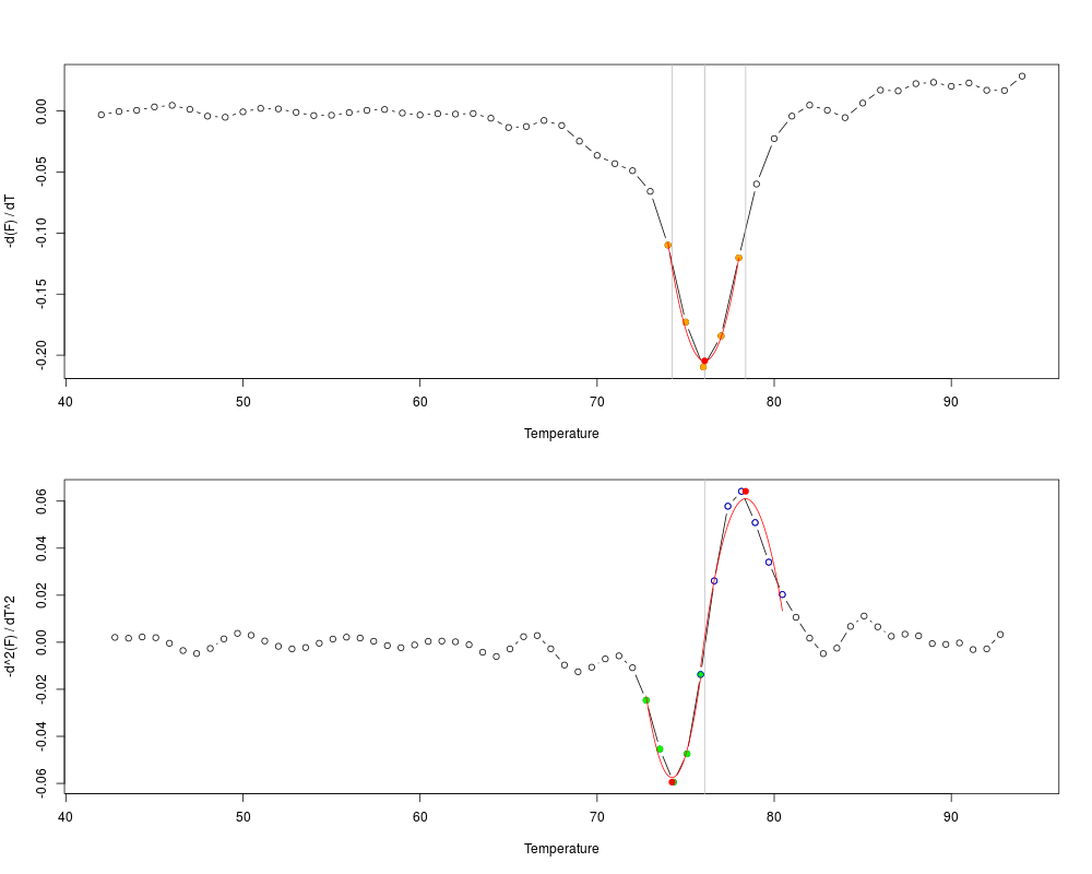
# First Example
# Plot the first and the second derivative melting curves of MLC-2v
# for a single melting curve. Should give a warning message but the graph
# will show you that the calculation is ok
data(MultiMelt)
tmp <- mcaSmoother(MultiMelt[, 1], MultiMelt[, 14])
diffQ2(tmp, fct = min, verbose = FALSE, plot = TRUE)
# Second Example
# Calculate the maximum fluorescence of a melting curve, Tm,
# Tm1D2 and Tm2D2 of HPRT1 for 12 microbead populations and assign the
# values to the matrix HPRT1
data(MultiMelt)
HPRT1 <- matrix(NA,12,4,
dimnames = list(colnames(MultiMelt[, 2L:13]),
c("Fluo", "Tm", "Tm1D2", "Tm2D2")))
for (i in 2L:13) {
tmp <- mcaSmoother(MultiMelt[, 1],
MultiMelt[, i])
tmpTM <- diffQ2(tmp, fct = min, verbose = TRUE)
HPRT1[i-1, 1] <- max(tmp$y)
HPRT1[i-1, 2] <- tmpTM$TmD1$Tm
HPRT1[i-1, 3] <- tmpTM$Tm1D2$Tm
HPRT1[i-1, 4] <- tmpTM$Tm2D2$Tm
}
HPRT1
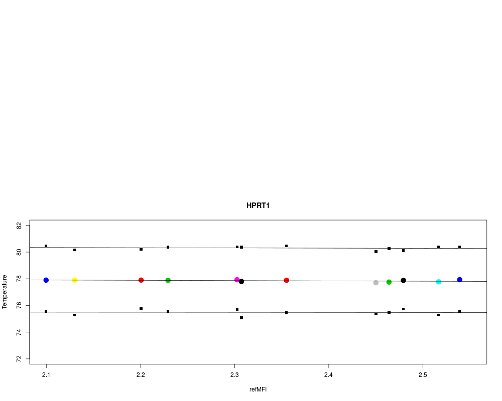
# Third Example
# Use diffQ2 to determine the second derivative.
data(MultiMelt)
HPRT1 <- matrix(NA,12,4,
dimnames = list(colnames(MultiMelt[, 2L:13]),
c("Fluo", "Tm", "Tm1D2", "Tm2D2")))
for (i in 2L:13) {
tmp <- mcaSmoother(MultiMelt[, 1],
MultiMelt[, i])
tmpTM <- diffQ2(tmp, fct = min, verbose = TRUE)
HPRT1[i-1, 1] <- max(tmp[["y.sp"]])
HPRT1[i-1, 2] <- tmpTM[["TmD1"]][["Tm"]]
HPRT1[i-1, 3] <- tmpTM[["Tm1D2"]][["Tm"]]
HPRT1[i-1, 4] <- tmpTM[["Tm2D2"]][["Tm"]]
}
plot(HPRT1[, 1], HPRT1[, 2],
xlab = "refMFI", ylab = "Temperature",
main = "HPRT1", xlim = c(2.1,2.55),
ylim = c(72,82), pch = 19,
col = 1:12, cex = 1.8)
points(HPRT1[, 1], HPRT1[, 3], pch = 15)
points(HPRT1[, 1], HPRT1[, 4], pch = 15)
abline(lm(HPRT1[, 2] ~ HPRT1[, 1]))
abline(lm(HPRT1[, 3] ~ HPRT1[, 1]))
abline(lm(HPRT1[, 4] ~ HPRT1[, 1]))
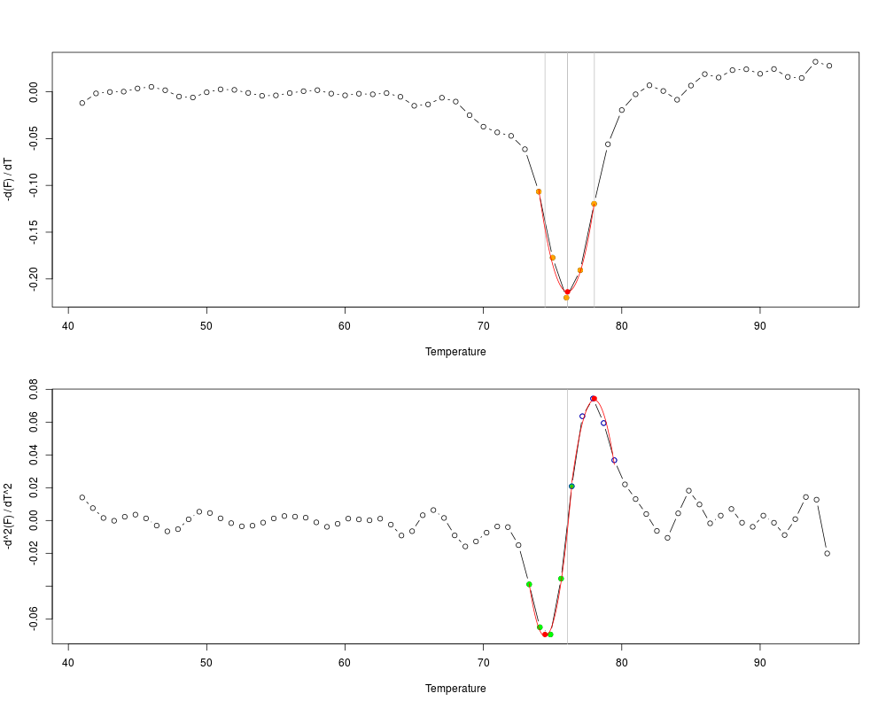
# Fourth Example
# Use diffQ2 with inder parameter to determine the second derivative.
data(MultiMelt)
tmp <- mcaSmoother(MultiMelt[, 1], MultiMelt[, 14])
diffQ2(tmp, fct = min, verbose = FALSE, plot = TRUE, inder = FALSE)
diffQ2(tmp, fct = min, verbose = FALSE, plot = TRUE, inder = TRUE)
par(mfrow = c(1,1))
Results
R version 3.3.1 (2016-06-21) -- "Bug in Your Hair"
Copyright (C) 2016 The R Foundation for Statistical Computing
Platform: x86_64-pc-linux-gnu (64-bit)

R is free software and comes with ABSOLUTELY NO WARRANTY.
You are welcome to redistribute it under certain conditions.
Type 'license()' or 'licence()' for distribution details.

R is a collaborative project with many contributors.
Type 'contributors()' for more information and
'citation()' on how to cite R or R packages in publications.

Type 'demo()' for some demos, 'help()' for on-line help, or
'help.start()' for an HTML browser interface to help.
Type 'q()' to quit R.

> library(MBmca)
Loading required package: robustbase
Loading required package: chipPCR
> png(filename="/home/ddbj/snapshot/RGM3/R_CC/result/MBmca/diffQ2.Rd_%03d_medium.png", width=480, height=480)
> ### Name: diffQ2
> ### Title: Calculation of the melting temperatures (Tm, Tm1D2 and Tm2D2)
> ###   from the first and the second derivative
> ### Aliases: diffQ2
> ### Keywords: Tm
>
> ### ** Examples
>
> # First Example
> # Plot the first and the second derivative melting curves of MLC-2v
> # for a single melting curve. Should give a warning message but the graph
> # will show you that the calculation is ok
> data(MultiMelt)
> tmp <- mcaSmoother(MultiMelt[, 1], MultiMelt[, 14])
> diffQ2(tmp, fct = min, verbose = FALSE, plot = TRUE)
Calculated Tm: 76.07117
Signal height at calculated Tm: -0.2046684
Calculated 'left' Tm: 74.22829
Calculated 'left' signal height: -0.05752853
Calculated 'right' Tm: 78.38657
Calculated 'right' signal height: 0.06101161
>
> # Second Example
> # Calculate the maximum fluorescence of a melting curve, Tm,
> # Tm1D2 and Tm2D2 of HPRT1 for 12 microbead populations and assign the
> # values to the matrix HPRT1
> data(MultiMelt)
> HPRT1 <- matrix(NA,12,4,
+ 	dimnames = list(colnames(MultiMelt[, 2L:13]),
+ 	    c("Fluo", "Tm", "Tm1D2", "Tm2D2")))
> for (i in 2L:13) {
+        tmp <- mcaSmoother(MultiMelt[, 1],
+                      MultiMelt[, i])
+        tmpTM <- diffQ2(tmp, fct = min, verbose = TRUE)
+        HPRT1[i-1, 1] <- max(tmp$y)
+        HPRT1[i-1, 2] <- tmpTM$TmD1$Tm
+        HPRT1[i-1, 3] <- tmpTM$Tm1D2$Tm
+        HPRT1[i-1, 4] <- tmpTM$Tm2D2$Tm
+ }
> HPRT1
             Fluo       Tm    Tm1D2    Tm2D2
HPRT1.1  2.479344 77.88494 75.74357 80.11672
HPRT1.2  2.200499 77.90029 75.75822 80.20735
HPRT1.3  2.464025 77.75343 75.48246 80.26107
HPRT1.4  2.099466 77.89949 75.54436 80.47610
HPRT1.5  2.516786 77.76936 75.29387 80.38587
HPRT1.6  2.302487 77.93054 75.69302 80.39532
HPRT1.7  2.129861 77.90438 75.28747 80.17770
HPRT1.8  2.450089 77.70170 75.35747 80.03902
HPRT1.9  2.307141 77.79736 75.08218 80.37068
HPRT1.10 2.355077 77.88993 75.45751 80.47056
HPRT1.11 2.229069 77.88330 75.57044 80.37306
HPRT1.12 2.539186 77.93199 75.55274 80.39795
>
> # Third Example
> # Use diffQ2 to determine the second derivative.
>
> data(MultiMelt)
> HPRT1 <- matrix(NA,12,4,
+ 	dimnames = list(colnames(MultiMelt[, 2L:13]),
+ 	    c("Fluo", "Tm", "Tm1D2", "Tm2D2")))
> for (i in 2L:13) {
+        tmp <- mcaSmoother(MultiMelt[, 1],
+                      MultiMelt[, i])
+        tmpTM <- diffQ2(tmp, fct = min, verbose = TRUE)
+        HPRT1[i-1, 1] <- max(tmp[["y.sp"]])
+        HPRT1[i-1, 2] <- tmpTM[["TmD1"]][["Tm"]]
+        HPRT1[i-1, 3] <- tmpTM[["Tm1D2"]][["Tm"]]
+        HPRT1[i-1, 4] <- tmpTM[["Tm2D2"]][["Tm"]]
+ }
> plot(HPRT1[, 1], HPRT1[, 2],
+        xlab = "refMFI", ylab = "Temperature",
+        main = "HPRT1", xlim = c(2.1,2.55),
+        ylim = c(72,82), pch = 19,
+        col = 1:12, cex = 1.8)
> points(HPRT1[, 1], HPRT1[, 3], pch = 15)
> points(HPRT1[, 1], HPRT1[, 4], pch = 15)
> abline(lm(HPRT1[, 2] ~ HPRT1[, 1]))
> abline(lm(HPRT1[, 3] ~ HPRT1[, 1]))
> abline(lm(HPRT1[, 4] ~ HPRT1[, 1]))
>
> # Fourth Example
> # Use diffQ2 with inder parameter to determine the second derivative.
> data(MultiMelt)
>
> tmp <- mcaSmoother(MultiMelt[, 1], MultiMelt[, 14])
> diffQ2(tmp, fct = min, verbose = FALSE, plot = TRUE, inder = FALSE)
Calculated Tm: 76.07117
Signal height at calculated Tm: -0.2046684
Calculated 'left' Tm: 74.22829
Calculated 'left' signal height: -0.05752853
Calculated 'right' Tm: 78.38657
Calculated 'right' signal height: 0.06101161
> diffQ2(tmp, fct = min, verbose = FALSE, plot = TRUE, inder = TRUE)
Calculated Tm: 76.07755
Signal height at calculated Tm: -0.2137656
Calculated 'left' Tm: 74.45108
Calculated 'left' signal height: -0.07054002
Calculated 'right' Tm: 78.01791
Calculated 'right' signal height: 0.07352439
> par(mfrow = c(1,1))
>
>
>
>
>
> dev.off()
null device
          1
>
 .
.