Function to pre-process melting curve data.

Description

The function mcaSmoother() is used for data pre-processing. Measurements from experimental systems may occasionally include missing values (NA). mcaSmoother() uses approx() to fill up NAs under the assumption that all measurements were equidistant. The original data remain unchanged and only the NAs are substituted. Following it calls smooth.spline() to smooth the curve. Different strengths can be set using the option df.fact (f default~0.95). Internally it takes the degree of freedom value from the spline and multiplies it with a factor between 0.6 and 1.1. Values lower than 1 result in stronger smoothed curves. The outcome of the differentiation depends on the temperature resolution of the melting curve. It is recommended to use a temperature resolution of at least 0.5 degree Celsius. In addition equal distances (e.g., 50 -> 50.5 -> 60 degree Celsius) rather than unequal distances (e.g., 50 -> 50.4 -> 60.1 degree Celsius) for the temperature steps are recommended. The parameter n can be used to increase the temperature resolution of the melting curve data. mcaSmoother uses the spline function for this purpose. A temperature range for a simple linear background correction. The linear trend is estimated by a robust linear regression using lmrob(). In case criteria for a robust linear regression are violated lm() is automatically used. The parameter n can be combined with the parameter Trange to make transform all melting curves of question to have the #same range and similar resolution. Optionally a Min-Max normalization between 0 and 1 can be used by setting the option minmax to TRUE. This is useful in many situations. For example, if the fluorescence values between samples vary considerably (e.g., due to high background, different reporter dyes,...), particularly in solution or for better comparison of results.

Usage

mcaSmoother(x, y, bgadj = FALSE, bg = NULL, Trange = NULL,
  minmax = FALSE, df.fact = 0.95, n = NULL)

Arguments

Value

Author(s)

Stefan Roediger

References

A Highly Versatile Microscope Imaging Technology Platform for the Multiplex Real-Time Detection of Biomolecules and Autoimmune Antibodies. S. Roediger, P. Schierack, A. Boehm, J. Nitschke, I. Berger, U. Froemmel, C. Schmidt, M. Ruhland, I. Schimke, D. Roggenbuck, W. Lehmann and C. Schroeder. Advances in Biochemical Bioengineering/Biotechnology. 133:33–74, 2013. http://www.ncbi.nlm.nih.gov/pubmed/22437246

Nucleic acid detection based on the use of microbeads: a review. S. Roediger, C. Liebsch, C. Schmidt, W. Lehmann, U. Resch-Genger, U. Schedler, P. Schierack. Microchim Acta 2014:1–18. DOI: 10.1007/s00604-014-1243-4

Roediger S, Boehm A, Schimke I. Surface Melting Curve Analysis with R. The R Journal 2013;5:37–53.

See Also

MFIerror, lmrob, smooth.spline, spline, lm, approx

Examples

# First Example
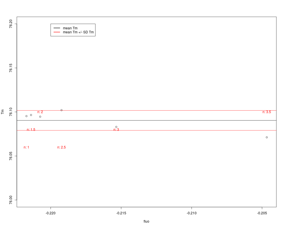
# Use mcaSmoother with different n to increase the temperature
# resolution of the melting curve artificially. Compare the
# influence of the n on the Tm and fluoTm values
data(MultiMelt)

Tm	<- vector()
fluo	<- vector()
for (i in seq(1,3.5,0.5)) {
  res.smooth <- mcaSmoother(MultiMelt[, 1], MultiMelt[, 14], n = i)
  res <- diffQ(res.smooth)
  Tm <- c(Tm, res$Tm)
  fluo <- c(fluo, res$fluoTm)
}
plot(fluo, Tm, ylim = c(76,76.2))
abline(h = mean(Tm))
text(fluo, seq(76.1,76.05,-0.02),
      paste("n:", seq(3.5,1,-0.5), sep = " "), col = 2)
abline(h = c(mean(Tm) + sd(Tm), mean(Tm) - sd(Tm)), col = 2)

legend(-0.22, 76.2, c("mean Tm", "mean Tm +/- SD Tm"),
	col = c(1,2), lwd = 2)

# Second Example
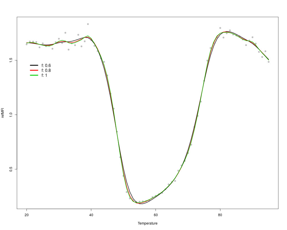
# Use mcaSmoother with different strengths of smoothing
# (f, 0.6 = strongest, 1 = weakest).
data(DMP)
plot(DMP[, 1], DMP[,6],
      xlim = c(20,95), xlab = "Temperature",
      ylab = "refMFI", pch = 19, col = 8)
f <- c(0.6, 0.8, 1.0)
for (i in c(1:3)) {
 	lines(mcaSmoother(DMP[, 1],
         DMP[,6], df.fact = f[i]),
         col = i, lwd = 2)
}
legend(20, 1.5, paste("f", f, sep = ": "),
      cex = 1.2, col =  1:3, bty = "n",
      lty = 1, lwd = 4)

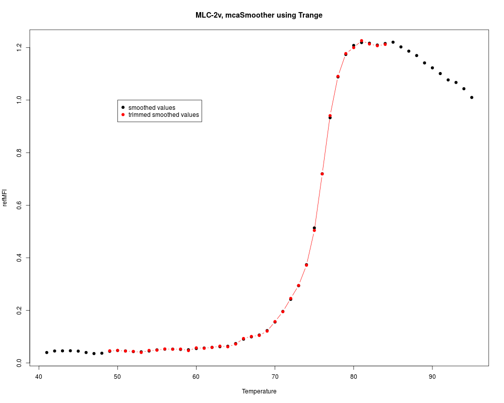
# Third Example
# Plot the smoothed and trimmed melting curve
data(MultiMelt)
tmp <- mcaSmoother(MultiMelt[, 1], MultiMelt[, 14])
tmp.trimmed <- mcaSmoother(MultiMelt[, 1], MultiMelt[, 14],
			    Trange = c(49,85))
plot(tmp, pch = 19, xlab = "Temperature", ylab = "refMFI",
	  main = "MLC-2v, mcaSmoother using Trange")
  points(tmp.trimmed, col = 2, type = "b", pch = 19)
  legend(50, 1, c("smoothed values",
		  "trimmed smoothed values"),
		   pch = c(19,19), col = c(1,2))

# Fourth Example
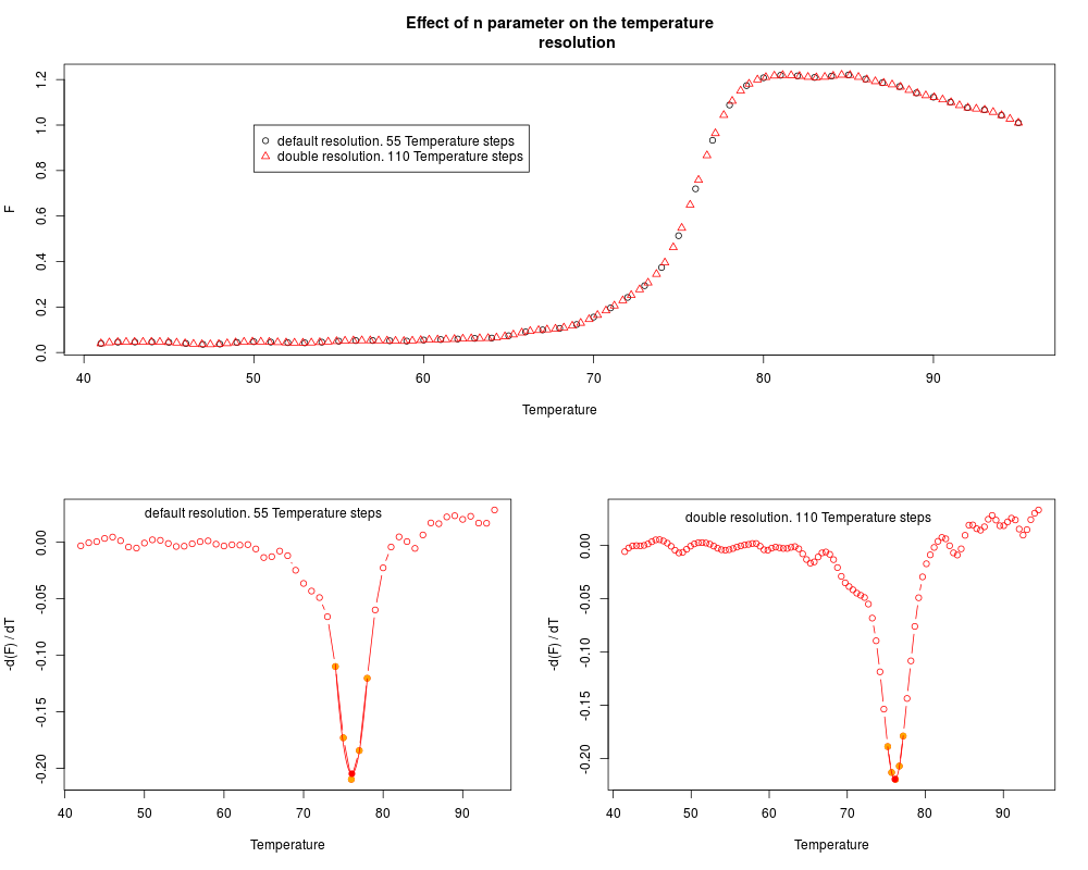
# Use mcaSmoother with different n to increase the temperature
# resolution of the melting curve. Caution, this operation may
# affect your data negatively if the resolution is set to high.
# Higher resolutions will just give the impression of better
# data quality. res.st uses the default resolution (no
# alteration)
# res.high uses the double resolution.
data(MultiMelt)
res.st <- mcaSmoother(MultiMelt[, 1], MultiMelt[, 14])
res.high <- mcaSmoother(MultiMelt[, 1], MultiMelt[, 14], n = 2)

par(fig = c(0,1,0.5,1))
plot(res.st, xlab = "Temperature", ylab = "F",
	main = "Effect of n parameter on the temperature
	resolution")
points(res.high, col = 2, pch = 2)
  legend(50, 1, c(paste("default resolution.", nrow(res.st),
		  "Temperature steps", sep = " "),
		  paste("double resolution.", nrow(res.high),
		  "Temperature steps", sep = " ")),
		  pch = c(1,2), col = c(1,2))
par(fig = c(0,0.5,0,0.5), new  =  TRUE)
diffQ(res.st, plot = TRUE)
  text(65, 0.025, paste("default resolution.", nrow(res.st),
			"Temperature steps", sep = " "))
par(fig = c(0.5,1,0,0.5), new = TRUE)
diffQ(res.high, plot = TRUE)
  text(65, 0.025, paste("double resolution.", nrow(res.high),
			"Temperature steps", sep = " "))

# Fifth example
# Different experiments may have different temperature
# resolutions and temperature ranges. The example uses a
# simulated melting curve with a temperature resolution of
# 0.5 and 1 degree Celsius and a temperature range of
# 35 to 95 degree Celsius.
#
# Coefficients of a 3 parameter sigmoid model.  Note:
# The off-set, temperature range and temperature resolution
# differ between both simulations. However, the melting
# temperatures should be very
# similar finally.
b <- -0.5; e <- 77

# Simulate first melting curve with a temperature
# between 35 - 95 degree Celsius and 1 degree Celsius
# per step temperature resolution.

t1 <- seq(35, 95, 1)
f1 <- 0.3 + 4 / (1 + exp(b * (t1 - e)))

# Simulate second melting curve with a temperature
# between 41.5 - 92.1 degree Celsius and 0.5 degree Celsius
# per step temperature resolution.
t2 <- seq(41.5, 92.1, 0.5)
f2 <- 0.2 + 2 / (1 + exp(b * (t2 - e)))

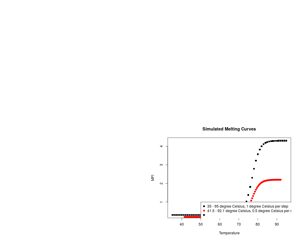
# Plot both simulated melting curves
plot(t1, f1, pch = 15, ylab = "MFI",
     main = "Simulated Melting Curves",
     xlab = "Temperature", col = 1)
points(t2, f2, pch = 19, col = 2)
legend(50, 1,
       c("35 - 95 degree Celsius, 1 degree Celsius per step",
       "41.5 - 92.1 degree Celsius, 0.5 degree Celsius per step",
       sep = " "), pch = c(15,19), col = c(1,2))

# Use mcaSmoother with n = 2 to increase the temperature
# resolution of the first simulated melting curve. The minmax
# parameter is used to make the peak heights compareable. The
# temperature range was limited between 45 to 90 degree Celsius for
# both simulations

t1f1 <- mcaSmoother(t1, f1, Trange= c(45, 90), minmax = TRUE, n = 2)
t2f2 <- mcaSmoother(t2, f2, Trange= c(45, 90), minmax = TRUE, n = 1)

# Perform a MCA on both altered simulations. As expected, the melting
# temperature are almost identical.
par(mfrow = c(2,1))
# Tm 77.00263, fluoTm -0.1245848
diffQ(t1f1, plot = TRUE)
text(60, -0.08,
     "Raw data: 35 - 95 degree Celsius,\n 1 degree Celsius per step")

# Tm 77.00069, fluoTm -0.1245394
diffQ(t2f2, plot = TRUE)
text(60, -0.08, "Raw data: 41.5 - 92.1 degree Celsius,
      \n 0.5 degree Celsius per step")
par(mfrow = c(1,1))

Results

R version 3.3.1 (2016-06-21) -- "Bug in Your Hair"
Copyright (C) 2016 The R Foundation for Statistical Computing
Platform: x86_64-pc-linux-gnu (64-bit)

R is free software and comes with ABSOLUTELY NO WARRANTY.
You are welcome to redistribute it under certain conditions.
Type 'license()' or 'licence()' for distribution details.

R is a collaborative project with many contributors.
Type 'contributors()' for more information and
'citation()' on how to cite R or R packages in publications.

Type 'demo()' for some demos, 'help()' for on-line help, or
'help.start()' for an HTML browser interface to help.
Type 'q()' to quit R.

> library(MBmca)
Loading required package: robustbase
Loading required package: chipPCR
> png(filename="/home/ddbj/snapshot/RGM3/R_CC/result/MBmca/mcaSmoother.Rd_%03d_medium.png", width=480, height=480)
> ### Name: mcaSmoother
> ### Title: Function to pre-process melting curve data.
> ### Aliases: mcaSmoother
> ### Keywords: background normalization smooth
> 
> ### ** Examples
> 
> # First Example
> # Use mcaSmoother with different n to increase the temperature
> # resolution of the melting curve artificially. Compare the
> # influence of the n on the Tm and fluoTm values
> data(MultiMelt)
> 
> Tm	<- vector()
> fluo	<- vector()
> for (i in seq(1,3.5,0.5)) {
+   res.smooth <- mcaSmoother(MultiMelt[, 1], MultiMelt[, 14], n = i)
+   res <- diffQ(res.smooth)
+   Tm <- c(Tm, res$Tm)
+   fluo <- c(fluo, res$fluoTm)
+ }
> plot(fluo, Tm, ylim = c(76,76.2))
> abline(h = mean(Tm))
> text(fluo, seq(76.1,76.05,-0.02),
+       paste("n:", seq(3.5,1,-0.5), sep = " "), col = 2)
> abline(h = c(mean(Tm) + sd(Tm), mean(Tm) - sd(Tm)), col = 2)
> 
> legend(-0.22, 76.2, c("mean Tm", "mean Tm +/- SD Tm"),
+ 	col = c(1,2), lwd = 2)
> 
> # Second Example
> # Use mcaSmoother with different strengths of smoothing
> # (f, 0.6 = strongest, 1 = weakest).
> data(DMP)
> plot(DMP[, 1], DMP[,6],
+       xlim = c(20,95), xlab = "Temperature",
+       ylab = "refMFI", pch = 19, col = 8)
> f <- c(0.6, 0.8, 1.0)
> for (i in c(1:3)) {
+  	lines(mcaSmoother(DMP[, 1],
+          DMP[,6], df.fact = f[i]),
+          col = i, lwd = 2)
+ }
> legend(20, 1.5, paste("f", f, sep = ": "),
+       cex = 1.2, col =  1:3, bty = "n",
+       lty = 1, lwd = 4)
> 
> # Third Example
> # Plot the smoothed and trimmed melting curve
> data(MultiMelt)
> tmp <- mcaSmoother(MultiMelt[, 1], MultiMelt[, 14])
> tmp.trimmed <- mcaSmoother(MultiMelt[, 1], MultiMelt[, 14],
+ 			    Trange = c(49,85))
> plot(tmp, pch = 19, xlab = "Temperature", ylab = "refMFI",
+ 	  main = "MLC-2v, mcaSmoother using Trange")
>   points(tmp.trimmed, col = 2, type = "b", pch = 19)
>   legend(50, 1, c("smoothed values",
+ 		  "trimmed smoothed values"),
+ 		   pch = c(19,19), col = c(1,2))
> 
> # Fourth Example
> # Use mcaSmoother with different n to increase the temperature
> # resolution of the melting curve. Caution, this operation may
> # affect your data negatively if the resolution is set to high.
> # Higher resolutions will just give the impression of better
> # data quality. res.st uses the default resolution (no
> # alteration)
> # res.high uses the double resolution.
> data(MultiMelt)
> res.st <- mcaSmoother(MultiMelt[, 1], MultiMelt[, 14])
> res.high <- mcaSmoother(MultiMelt[, 1], MultiMelt[, 14], n = 2)
> 
> par(fig = c(0,1,0.5,1))
> plot(res.st, xlab = "Temperature", ylab = "F",
+ 	main = "Effect of n parameter on the temperature
+ 	resolution")
> points(res.high, col = 2, pch = 2)
>   legend(50, 1, c(paste("default resolution.", nrow(res.st),
+ 		  "Temperature steps", sep = " "),
+ 		  paste("double resolution.", nrow(res.high),
+ 		  "Temperature steps", sep = " ")),
+ 		  pch = c(1,2), col = c(1,2))
> par(fig = c(0,0.5,0,0.5), new  =  TRUE)
> diffQ(res.st, plot = TRUE)
Calculated Tm: 76.07117 
Signal height at calculated Tm: -0.2046684 
>   text(65, 0.025, paste("default resolution.", nrow(res.st),
+ 			"Temperature steps", sep = " "))
> par(fig = c(0.5,1,0,0.5), new = TRUE)
> diffQ(res.high, plot = TRUE)
Calculated Tm: 76.10204 
Signal height at calculated Tm: -0.2192319 
>   text(65, 0.025, paste("double resolution.", nrow(res.high),
+ 			"Temperature steps", sep = " "))
> 
> # Fifth example
> # Different experiments may have different temperature
> # resolutions and temperature ranges. The example uses a
> # simulated melting curve with a temperature resolution of
> # 0.5 and 1 degree Celsius and a temperature range of
> # 35 to 95 degree Celsius.
> #
> # Coefficients of a 3 parameter sigmoid model.  Note:
> # The off-set, temperature range and temperature resolution
> # differ between both simulations. However, the melting
> # temperatures should be very
> # similar finally.
> b <- -0.5; e <- 77
> 
> # Simulate first melting curve with a temperature
> # between 35 - 95 degree Celsius and 1 degree Celsius
> # per step temperature resolution.
> 
> t1 <- seq(35, 95, 1)
> f1 <- 0.3 + 4 / (1 + exp(b * (t1 - e)))
> 
> # Simulate second melting curve with a temperature
> # between 41.5 - 92.1 degree Celsius and 0.5 degree Celsius
> # per step temperature resolution.
> t2 <- seq(41.5, 92.1, 0.5)
> f2 <- 0.2 + 2 / (1 + exp(b * (t2 - e)))
> 
> # Plot both simulated melting curves
> plot(t1, f1, pch = 15, ylab = "MFI",
+      main = "Simulated Melting Curves",
+      xlab = "Temperature", col = 1)
> points(t2, f2, pch = 19, col = 2)
> legend(50, 1,
+        c("35 - 95 degree Celsius, 1 degree Celsius per step",
+        "41.5 - 92.1 degree Celsius, 0.5 degree Celsius per step",
+        sep = " "), pch = c(15,19), col = c(1,2))
> 
> # Use mcaSmoother with n = 2 to increase the temperature
> # resolution of the first simulated melting curve. The minmax
> # parameter is used to make the peak heights compareable. The
> # temperature range was limited between 45 to 90 degree Celsius for
> # both simulations
> 
> t1f1 <- mcaSmoother(t1, f1, Trange= c(45, 90), minmax = TRUE, n = 2)
> t2f2 <- mcaSmoother(t2, f2, Trange= c(45, 90), minmax = TRUE, n = 1)
> 
> # Perform a MCA on both altered simulations. As expected, the melting
> # temperature are almost identical.
> par(mfrow = c(2,1))
> # Tm 77.00263, fluoTm -0.1245848
> diffQ(t1f1, plot = TRUE)
Calculated Tm: 77.00263 
Signal height at calculated Tm: -0.1245848 
> text(60, -0.08,
+      "Raw data: 35 - 95 degree Celsius,\n 1 degree Celsius per step")
> 
> # Tm 77.00069, fluoTm -0.1245394
> diffQ(t2f2, plot = TRUE)
Calculated Tm: 77.00069 
Signal height at calculated Tm: -0.1245394 
> text(60, -0.08, "Raw data: 41.5 - 92.1 degree Celsius,
+       \n 0.5 degree Celsius per step")
> par(mfrow = c(1,1))
> 
> 
> 
> 
> 
> dev.off()
null device 
          1 
>