R Graphical Manual

Browse All

Last data update: 2014.03.03

R: Analyzes multivariate counts data using poisson-lognormal...

mcmc.otu

R Documentation

Analyzes multivariate counts data using poisson-lognormal mixed model

Description

Wrapper function for MCMCglmm by Jarrod Hadfield, designed for multivariate counts data such as in sequence-based analysis of microbial communities ("metabarcoding", variables = operational taxonomic units, OTUs), or in ecological applications (variables = species). The function aims to infer the changes in relative proportions of individual variables. The maximum number of variables that can be processed on a laptop computer is about 200; more memory is required for larger numbers.

Usage

mcmc.otu(fixed=NULL, random=NULL, data, y.scale="proportion", 
globalMainEffects="remove", vprior="uninf",...)

Arguments

`fixed`	combination of fixed effects, as a text string. Do not use "*" symbol, list it fully, such as: 'factor1+factor2+factor1:factor2'.
`random`	A vector of names for variable-specific scalar random effects, such as 'c("effect1","effect2")'.
`data`	output of the otuStack() function
`y.scale`	By default, the modeled abundances will be expressed relative to the total counts in the sample, effectively corresponding to proportions of total. Specify 'y.scale="absolute"' to express the results as absolute abundances.
`globalMainEffects`	By default, the model will assume that the samples can vary systematically in abundance among factor combinations (i.e., there is an effect of a factor combination applicable to all variables) and remove these effects; this is analogous to normalizing the samples to total counts. Specify 'globalMainEffects="keep"' to switch this off.
`vprior`	Prior for variance of user-specified random effects. By default an inverse Wishart prior with assumed variance (V) at 1 and the degree of belief parameter (nu) at 0. With 'prior="iw"' and 'prior="iw01"' nu is the number of OTUs minus 0.998, resulting in a weakly informative prior that is commonly used in this type of inference. vprior="iw" will assume large prior variance (1), vprior="iw01" will assume small prior variance (0.1). If the model has trouble converging, specify vptior="iw".
`...`	other options for MCMCglmm function, such as nitt (number of iterations), thin (tinning interval), and burnin (number of initial iterations to disregard). For a more precise inference, specify 'nitt=50000, thin=25, burnin=5000'. See MCMCglmm documentation for more details.

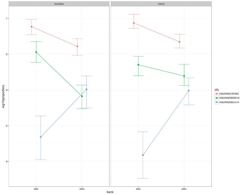
Details

This function constructs priors and runs an MCMC chain to fit a Poisson-lognormal generalized linear mixed model to the multivariate counts data.

The fixed effects for the model by default include a variable-specific intercept, global (non-variable-specific) main effects of fixed factors, and variable-specific effect for each of the listed fixed factors. With globalMainEffects="keep" the model will not include the global main effects, resulting in them being absorbed into the variable-specific effects.

The user-specified random effects are all assumed to be variable-specific with no covariances.

The model includes one universal random factor: the scalar random effect of sample, which accounts for the unequal counting effort among samples.

Residual variances are assumed to be variable-specific with no covariances, with weakly informative inverse Wishart prior with variance=1 and nu=(number of variables)-0.998.

The priors for fixed effects are diffuse gaussians with a mean at 0 and very large variances (1e+8),

Value

An MCMCglmm object. OTUsummary() function within this package summaizes these data, calculates all variable-wise credible intervals and p-values, and plots the results either as line-point-whiskers graph or a bar-whiskers graph using ggplot2 functions.

OTUsummary() only works for experiments with a single multilevel factor or two fully crossed multilevel factors.

For more useful operations on MCMCglmm objects, such as posterior.mode(), HPDinterval(), and plot(), see documentation for MCMCglmm package.

Author(s)

Mikhail V. Matz, University of Texas at Austin <matz@utexas.edu>

References

Elizabeth A. Green, Sarah W. Davies, Mikhail V. Matz, Monica Medina Next-generation sequencing reveals cryptic Symbiodinium diversity within Orbicella faveolata and Orbicella franksi at the Flower Garden Banks, Gulf of Mexico. PeerJ 2014 https://peerj.com/preprints/246/

Examples

	
# Symbiodinium sp diversity in two coral species at two reefs (banks)
data(green.data)

# removing outliers
goods=purgeOutliers(
	data=green.data,
	count.columns=c(4:length(green.data[1,])),
	zero.cut=0.25 # remove this line for real analysis
)

# stacking the data table
gs=otuStack(
	data=goods,
	count.columns=c(4:length(goods[1,])),
	condition.columns=c(1:3)
	)

# fitting the model
mm=mcmc.otu(
	fixed="bank+species+bank:species",
	data=gs,
	nitt=3000,burnin=2000 # remove this line for real analysis!
	)

# selecting the OTUs that were modeled reliably
acpass=otuByAutocorr(mm,gs)

# calculating effect sizes and p-values:
ss=OTUsummary(mm,gs,summ.plot=FALSE)

# correcting for mutliple comparisons (FDR)
ss=padjustOTU(ss)

# getting significatly changing OTUs (FDR<0.05)
sigs=signifOTU(ss)

# plotting them
ss2=OTUsummary(mm,gs,otus=sigs)

# bar-whiskers graph of relative changes:
# ssr=OTUsummary(mm,gs,otus=signifOTU(ss),relative=TRUE)

# displaying effect sizes and p-values for significant OTUs
ss$otuWise[sigs]

Results


R version 3.3.1 (2016-06-21) -- "Bug in Your Hair"
Copyright (C) 2016 The R Foundation for Statistical Computing
Platform: x86_64-pc-linux-gnu (64-bit)

R is free software and comes with ABSOLUTELY NO WARRANTY.
You are welcome to redistribute it under certain conditions.
Type 'license()' or 'licence()' for distribution details.

R is a collaborative project with many contributors.
Type 'contributors()' for more information and
'citation()' on how to cite R or R packages in publications.

Type 'demo()' for some demos, 'help()' for on-line help, or
'help.start()' for an HTML browser interface to help.
Type 'q()' to quit R.

> library(MCMC.OTU)
Loading required package: MCMCglmm
Loading required package: Matrix
Loading required package: coda
Loading required package: ape
Loading required package: ggplot2
> png(filename="/home/ddbj/snapshot/RGM3/R_CC/result/MCMC.OTU/mcmc.otu.Rd_%03d_medium.png", width=480, height=480)
> ### Name: mcmc.otu
> ### Title: Analyzes multivariate counts data using poisson-lognormal mixed
> ###   model
> ### Aliases: mcmc.otu
> 
> ### ** Examples
> 
> 	
> # Symbiodinium sp diversity in two coral species at two reefs (banks)
> data(green.data)
> 
> # removing outliers
> goods=purgeOutliers(
+ 	data=green.data,
+ 	count.columns=c(4:length(green.data[1,])),
+ 	zero.cut=0.25 # remove this line for real analysis
+ )
[1] "samples with counts below z-score -2.5 :"
[1] "EFAV153"
[1] "zscores:"
  EFAV153 
-3.884085 
[1] "OTUs passing frequency cutoff  0.001 : 10"
[1] "OTUs with counts in 0.25 of samples:"

FALSE  TRUE 
    3     7 
> 
> # stacking the data table
> gs=otuStack(
+ 	data=goods,
+ 	count.columns=c(4:length(goods[1,])),
+ 	condition.columns=c(1:3)
+ 	)
> 
> # fitting the model
> mm=mcmc.otu(
+ 	fixed="bank+species+bank:species",
+ 	data=gs,
+ 	nitt=3000,burnin=2000 # remove this line for real analysis!
+ 	)
$PRIOR
$PRIOR$R
$PRIOR$R$V
     [,1] [,2] [,3] [,4] [,5] [,6] [,7] [,8]
[1,]    1    0    0    0    0    0    0    0
[2,]    0    1    0    0    0    0    0    0
[3,]    0    0    1    0    0    0    0    0
[4,]    0    0    0    1    0    0    0    0
[5,]    0    0    0    0    1    0    0    0
[6,]    0    0    0    0    0    1    0    0
[7,]    0    0    0    0    0    0    1    0
[8,]    0    0    0    0    0    0    0    1

$PRIOR$R$nu
[1] 7.02


$PRIOR$G
$PRIOR$G$G1
$PRIOR$G$G1$V
[1] 1

$PRIOR$G$G1$nu
[1] 0




$FIXED
[1] "count~otu+bank+species+bank:species+otu:bank+otu:species+otu:bank:species"

$RANDOM
[1] "~sample"


                       MCMC iteration = 0

 Acceptance ratio for liability set 1 = 0.000158

 Acceptance ratio for liability set 2 = 0.000351

 Acceptance ratio for liability set 3 = 0.000158

 Acceptance ratio for liability set 4 = 0.000456

 Acceptance ratio for liability set 5 = 0.000351

 Acceptance ratio for liability set 6 = 0.000614

 Acceptance ratio for liability set 7 = 0.000526

 Acceptance ratio for liability set 8 = 0.000596

                       MCMC iteration = 1000

 Acceptance ratio for liability set 1 = 0.210912

 Acceptance ratio for liability set 2 = 0.423807

 Acceptance ratio for liability set 3 = 0.220158

 Acceptance ratio for liability set 4 = 0.438754

 Acceptance ratio for liability set 5 = 0.348825

 Acceptance ratio for liability set 6 = 0.425474

 Acceptance ratio for liability set 7 = 0.365965

 Acceptance ratio for liability set 8 = 0.511228

                       MCMC iteration = 2000

 Acceptance ratio for liability set 1 = 0.298246

 Acceptance ratio for liability set 2 = 0.431333

 Acceptance ratio for liability set 3 = 0.300544

 Acceptance ratio for liability set 4 = 0.451298

 Acceptance ratio for liability set 5 = 0.380158

 Acceptance ratio for liability set 6 = 0.418035

 Acceptance ratio for liability set 7 = 0.369807

 Acceptance ratio for liability set 8 = 0.515895

                       MCMC iteration = 3000

 Acceptance ratio for liability set 1 = 0.306579

 Acceptance ratio for liability set 2 = 0.409737

 Acceptance ratio for liability set 3 = 0.344702

 Acceptance ratio for liability set 4 = 0.467754

 Acceptance ratio for liability set 5 = 0.421386

 Acceptance ratio for liability set 6 = 0.473860

 Acceptance ratio for liability set 7 = 0.392807

 Acceptance ratio for liability set 8 = 0.487088
> 
> # selecting the OTUs that were modeled reliably
> acpass=otuByAutocorr(mm,gs)
> 
> # calculating effect sizes and p-values:
> ss=OTUsummary(mm,gs,summ.plot=FALSE)
> 
> # correcting for mutliple comparisons (FDR)
> ss=padjustOTU(ss)
> 
> # getting significatly changing OTUs (FDR<0.05)
> sigs=signifOTU(ss)
> 
> # plotting them
> ss2=OTUsummary(mm,gs,otus=sigs)
> 
> # bar-whiskers graph of relative changes:
> # ssr=OTUsummary(mm,gs,otus=signifOTU(ss),relative=TRUE)
> 
> # displaying effect sizes and p-values for significant OTUs
> ss$otuWise[sigs]
$H35JRAZ01ATSK2
                           difference
pvalue                      bankeast:speciesfaveolata bankeast:speciesfranksi
  bankeast:speciesfaveolata                        NA             0.093735024
  bankeast:speciesfranksi                  0.90613905                      NA
  bankwest:speciesfaveolata                0.01610127             0.002081439
  bankwest:speciesfranksi                  0.06230476             0.021495976
                           difference
pvalue                      bankwest:speciesfaveolata bankwest:speciesfranksi
  bankeast:speciesfaveolata                -0.5357087             -0.43754870
  bankeast:speciesfranksi                  -0.6294437             -0.53128372
  bankwest:speciesfaveolata                        NA              0.09815997
  bankwest:speciesfranksi                   0.8680081                      NA

$H35JRAZ03DED1S
                           difference
pvalue                      bankeast:speciesfaveolata bankeast:speciesfranksi
  bankeast:speciesfaveolata                        NA            -0.283215449
  bankeast:speciesfranksi                 0.538077764                      NA
  bankwest:speciesfaveolata               0.001340834             0.003929306
  bankwest:speciesfranksi                 0.068454428             0.475318570
                           difference
pvalue                      bankwest:speciesfaveolata bankwest:speciesfranksi
  bankeast:speciesfaveolata                -1.2229092              -0.6187028
  bankeast:speciesfranksi                  -0.9396937              -0.3354874
  bankwest:speciesfaveolata                        NA               0.6042063
  bankwest:speciesfranksi                   0.0775155                      NA

$H35JRAZ03DJU1V
                           difference
pvalue                      bankeast:speciesfaveolata bankeast:speciesfranksi
  bankeast:speciesfaveolata                        NA            -0.612505860
  bankeast:speciesfranksi                  0.53807776                      NA
  bankwest:speciesfaveolata                0.02994505             0.001340834
  bankwest:speciesfranksi                  0.01610127             0.001444949
                           difference
pvalue                      bankwest:speciesfaveolata bankwest:speciesfranksi
  bankeast:speciesfaveolata                 1.3421433              1.25320798
  bankeast:speciesfranksi                   1.9546492              1.86571384
  bankwest:speciesfaveolata                        NA             -0.08893536
  bankwest:speciesfranksi                   0.9210835                      NA

> 
> 
> 
> 
> 
> 
> dev.off()
null device 
          1 
>