R Graphical Manual

Browse All

Last data update: 2014.03.03

R: Plotting fixed effects for all genes for a single combination...

HPDplot

R Documentation

Plotting fixed effects for all genes for a single combination of factors

Description

Calculates and plots posterior means with 95% credible intervals for specified fixed effects (or their combination) for all genes

Usage

HPDplot(model, factors, factors2 = NULL, ylimits = NULL, 
hpdtype = "w", inverse = F, jitter = 0, plot = T, grid = T, zero = T, ...)

Arguments

`model`	The output of mcmc.qpcr function.
`factors`	A vector of names of fixed effects of interest; see details.
`factors2`	A second vector of fixed effect names to be subtracted from the first; see details.
`ylimits`	Y-limits for the plot such as c(-3,6); autoscale by default.
`hpdtype`	Specify hpdtype="l" to plot the upper and lower 95% credible limits as a continuous dashed line across all genes. This is useful to compare credible intervals among several models on the same plot. By default (hpdtype="w") the limits are plotted as whiskers around each point.
`inverse`	Plot the inverse of the result.
`jitter`	For hpdtype="w", shifts the plotted values and whiskers by the specified distance along the x axis (reasonable jitter values are 0.15 or -0.15, for example). This helps plot several results (different models or factor combinations) on the same plot (use HPDpoints to add to existing plot)
`plot`	if plot = FALSE the function returns a table of calculated posterior modes, means, upper and lower 95% credible limits (all on log(2) scale), and two types of p-values: derived from Bayesian z-scores, and derived directly from MCMC sample. All such outputs for a given experiment should be concatenated with rbind and processed by padj.qpcr() function to adjust the p-values for multiple comparisons (disregarding the entries corresponding to control genes)
`grid`	Whether to draw vertical grid lines to separate genes.
`zero`	Whether to draw a horizontal line at 0.
`...`	Various plot() options; such as col (color of lines and symbols), pch (type of symbol), main (plot title) etc.

Details

Use summary(MCMCglmm object) first to see what fixed effect names are actually used in the output. For example, if summary shows:

gene1:conditionheat
gene2:conditionheat
....
gene1:timepointtwo
gene2:timepointtwo
....
gene1:conditionheat:timepointtwo
gene2:conditionheat:timepointtwo

, it is possible to specify factors="conditionheat" to plot only the effects of the heat.

If a vector of several fixed effect names is given, for example: factors=c("timepointtwo","treatmentheat:timepointtwo") the function will plot the posterior mean and credible interval for the sum of these effects.

If a second vector is also given, for example,
factors=c("f1","f2"), factors2=c("f3","f4")
the function will plot the difference between the sums of these two groups of factors. This is useful for pairwise analysis of differences in complicated designs.

Value

A plot or a table (plot = F).

Use the function HPDpoints() if you need to add graphs to already existing plot.

Author(s)

Mikhail V. Matz, UT Austin <matz@utexas.edu>

References

Matz MV, Wright RM, Scott JG (2013) No Control Genes Required: Bayesian Analysis of qRT-PCR Data. PLoS ONE 8(8): e71448. doi:10.1371/journal.pone.0071448

Examples


# loading Cq data and amplification efficiencies
data(coral.stress) 
data(amp.eff) 
# extracting a subset of data 
cs.short=subset(coral.stress, timepoint=="one")

genecolumns=c(5,6,16,17) # specifying columns corresponding to genes of interest
conditions=c(1:4) # specifying columns containing factors  

# calculating molecule counts and reformatting:
dd=cq2counts(data=cs.short,genecols=genecolumns,
condcols=conditions,effic=amp.eff,Cq1=37) 

# fitting the model
mm=mcmc.qpcr(
	fixed="condition",
	data=dd,
	controls=c("nd5","rpl11"),
	nitt=3000,burnin=2000 # remove this line when analyzing real data!
)

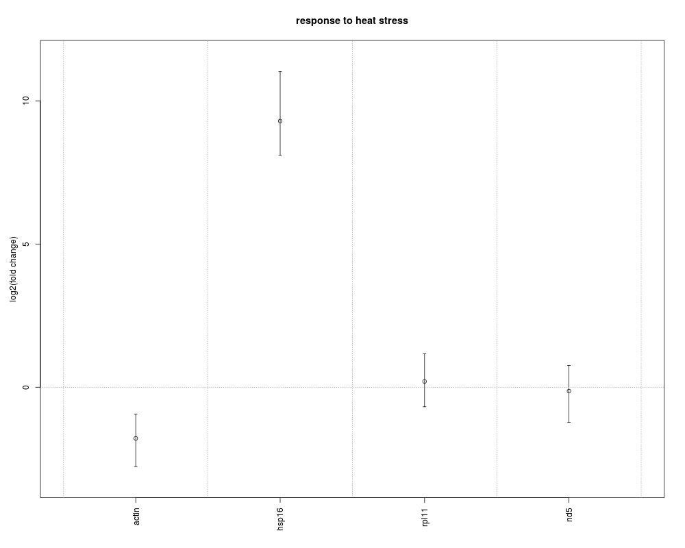
# plotting log2(fold change) in response to heat stress for all genes
HPDplot(model=mm,factors="conditionheat",main="response to heat stress")

Results


R version 3.3.1 (2016-06-21) -- "Bug in Your Hair"
Copyright (C) 2016 The R Foundation for Statistical Computing
Platform: x86_64-pc-linux-gnu (64-bit)

R is free software and comes with ABSOLUTELY NO WARRANTY.
You are welcome to redistribute it under certain conditions.
Type 'license()' or 'licence()' for distribution details.

R is a collaborative project with many contributors.
Type 'contributors()' for more information and
'citation()' on how to cite R or R packages in publications.

Type 'demo()' for some demos, 'help()' for on-line help, or
'help.start()' for an HTML browser interface to help.
Type 'q()' to quit R.

> library(MCMC.qpcr)
Loading required package: MCMCglmm
Loading required package: Matrix
Loading required package: coda
Loading required package: ape
Loading required package: ggplot2
> png(filename="/home/ddbj/snapshot/RGM3/R_CC/result/MCMC.qpcr/HPDplot.Rd_%03d_medium.png", width=480, height=480)
> ### Name: HPDplot
> ### Title: Plotting fixed effects for all genes for a single combination of
> ###   factors
> ### Aliases: HPDplot
> 
> ### ** Examples
> 
> 
> # loading Cq data and amplification efficiencies
> data(coral.stress) 
> data(amp.eff) 
> # extracting a subset of data 
> cs.short=subset(coral.stress, timepoint=="one")
> 
> genecolumns=c(5,6,16,17) # specifying columns corresponding to genes of interest
> conditions=c(1:4) # specifying columns containing factors  
> 
> # calculating molecule counts and reformatting:
> dd=cq2counts(data=cs.short,genecols=genecolumns,
+ condcols=conditions,effic=amp.eff,Cq1=37) 
> 
> # fitting the model
> mm=mcmc.qpcr(
+ 	fixed="condition",
+ 	data=dd,
+ 	controls=c("nd5","rpl11"),
+ 	nitt=3000,burnin=2000 # remove this line when analyzing real data!
+ )
$PRIOR
$PRIOR$B
$PRIOR$B$mu
[1] 0 0 0 0 0 0 0 0

$PRIOR$B$V
      [,1]  [,2]  [,3]  [,4]  [,5]  [,6]      [,7]      [,8]
[1,] 1e+08 0e+00 0e+00 0e+00 0e+00 0e+00 0.0000000 0.0000000
[2,] 0e+00 1e+08 0e+00 0e+00 0e+00 0e+00 0.0000000 0.0000000
[3,] 0e+00 0e+00 1e+08 0e+00 0e+00 0e+00 0.0000000 0.0000000
[4,] 0e+00 0e+00 0e+00 1e+08 0e+00 0e+00 0.0000000 0.0000000
[5,] 0e+00 0e+00 0e+00 0e+00 1e+08 0e+00 0.0000000 0.0000000
[6,] 0e+00 0e+00 0e+00 0e+00 0e+00 1e+08 0.0000000 0.0000000
[7,] 0e+00 0e+00 0e+00 0e+00 0e+00 0e+00 0.3663091 0.0000000
[8,] 0e+00 0e+00 0e+00 0e+00 0e+00 0e+00 0.0000000 0.3663091


$PRIOR$R
$PRIOR$R$V
     [,1] [,2] [,3] [,4]
[1,]    1    0    0    0
[2,]    0    1    0    0
[3,]    0    0    1    0
[4,]    0    0    0    1

$PRIOR$R$nu
[1] 3.002


$PRIOR$G
$PRIOR$G$G1
$PRIOR$G$G1$V
[1] 1

$PRIOR$G$G1$nu
[1] 0




$FIXED
[1] "count~0+gene++gene:condition"

$RANDOM
[1] "~sample"


                       MCMC iteration = 0

 Acceptance ratio for liability set 1 = 0.000438

 Acceptance ratio for liability set 2 = 0.000419

 Acceptance ratio for liability set 3 = 0.000226

 Acceptance ratio for liability set 4 = 0.000313

                       MCMC iteration = 1000

 Acceptance ratio for liability set 1 = 0.102625

 Acceptance ratio for liability set 2 = 0.380806

 Acceptance ratio for liability set 3 = 0.307387

 Acceptance ratio for liability set 4 = 0.115281

                       MCMC iteration = 2000

 Acceptance ratio for liability set 1 = 0.156406

 Acceptance ratio for liability set 2 = 0.425194

 Acceptance ratio for liability set 3 = 0.356710

 Acceptance ratio for liability set 4 = 0.174469

                       MCMC iteration = 3000

 Acceptance ratio for liability set 1 = 0.168875

 Acceptance ratio for liability set 2 = 0.420645

 Acceptance ratio for liability set 3 = 0.353129

 Acceptance ratio for liability set 4 = 0.194000
> 
> # plotting log2(fold change) in response to heat stress for all genes
> HPDplot(model=mm,factors="conditionheat",main="response to heat stress")
> 
> 
> 
> 
> 
> 
> dev.off()
null device 
          1 
>