R Graphical Manual

Browse All

Last data update: 2014.03.03

R: Plots qPCR analysis results for individual genes.

HPDplotBygene

R Documentation

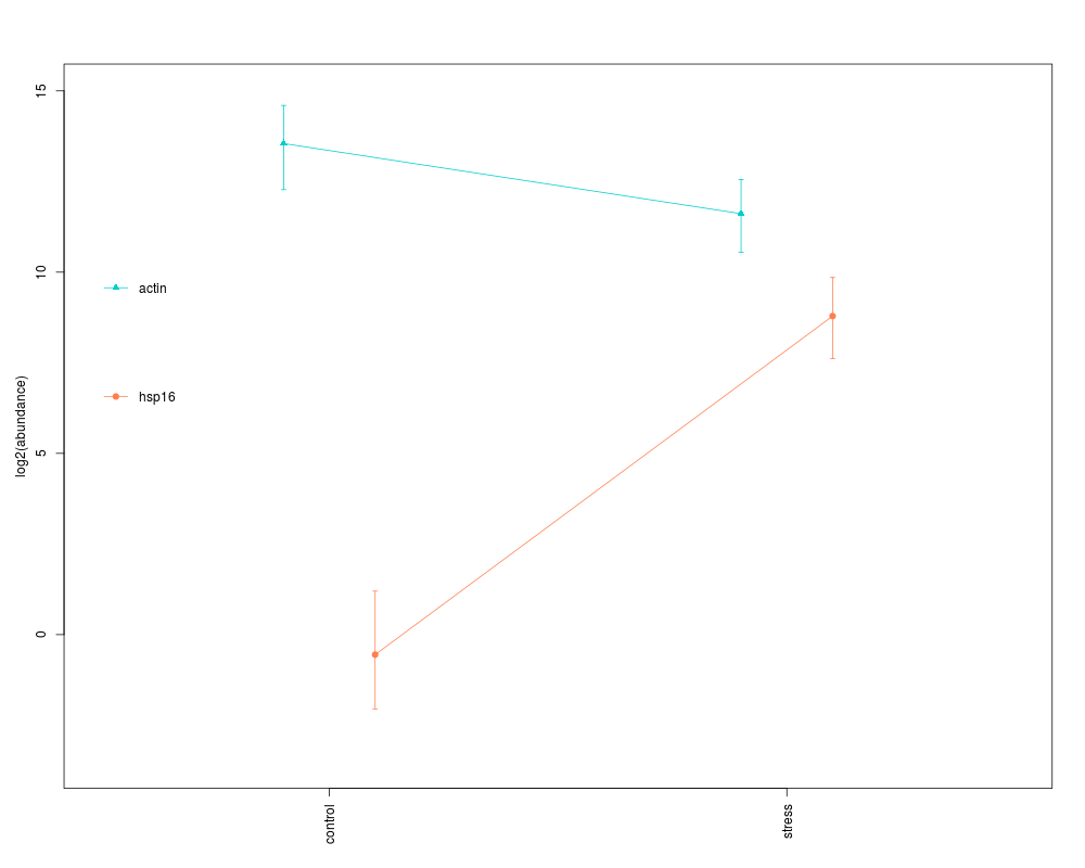
Plots qPCR analysis results for individual genes.

Description

For a particular gene, plots model-predicted values (and credible intervals) for a series of specified fixed effect combinations ("conditions").

Usage

HPDplotBygene(model, gene, conditions, pval = "mcmc", newplot = T, 
ylimits = NULL, inverse = F, jitter = 0, plot = T, yscale = "log2", 
interval = "ci", grid = F, zero = F, ...)

Arguments

`model`	model object produced by MCMC.qpcr()
`gene`	name of the gene to plot
`conditions`	A list naming the conditions to plot and defining them as combination of fixed effects (See example below). '0' denotes gene-specific intercept.
`pval`	Type of p-value to report: 'mcmc' - MCMC-based (default), 'z' - based on Bayesian z-score. Use 'z' to approximate p-values lower than 2/[MCMC sample size] (with default MCMC.qpcr settings, this comes to 0.002)
`newplot`	When TRUE, a new plot should be created. When FALSE, or a graph will be added to an existing plot.
`ylimits`	Y-limits for the plot such as c(-3,6); autoscale by default.
`inverse`	When TRUE, the inverse of the data will be plotted.
`jitter`	Shifts the plotted values and whiskers by the specified distance along the x axis (reasonable jitter values are 0.15 or -0.15, for example). This helps plot several graphs on the same plot without overlapping.
`plot`	When FALSE, no plot will be generated; the function will just list mean pairwise differences and p-values.
`yscale`	Scale on which to represent the data. In all mcmc.qpcr models the model scale is natural logarithm, which I prefer to translate into log2 or log10 (if the differences are orders of magnitude) for better human readability. The default is 'log2'; other options are 'log10' and 'native' (no rescaling of the model data). There is also a beta-option 'proportion', which is not useful for qPCR. It was added to cannibalize HPDplotBygene function for plotting results of the model operating with arcsin-square root transfromed proportions. With yscale="proportions", the plot will be on the original proportion scale but the tukey-like differences will still be reported on the asin(sqrt()) transformed scale.
`interval`	'ci' (default) will plot 95% credible limits of the posterior distribution, 'sd' will plot the mean plus/minus one standard deviation of the posterior.
`grid`	When TRUE, a vertical grid separating conditions will be added
`zero`	When TRUE, a y=0 line will be added.
`...`	Various plot() options.

Value

Generates a point-whiskers plot, lists pairwise mean differenes between all conditions, calculates and lists pairwise p-values (not corrected for multiple testing).

Author(s)

Mikhal V. Matz, UT Austin, matz@utexas.edu

References

Matz MV, Wright RM, Scott JG (2013) No Control Genes Required: Bayesian Analysis of qRT-PCR Data. PLoS ONE 8(8): e71448. doi:10.1371/journal.pone.0071448

Examples


# loading Cq data and amplification efficiencies
data(coral.stress) 
data(amp.eff) 
# extracting a subset of data 
cs.short=subset(coral.stress, timepoint=="one")

genecolumns=c(5,6,16,17) # specifying columns corresponding to genes of interest
conditions=c(1:4) # specifying columns containing factors  

# calculating molecule counts and reformatting:
dd=cq2counts(data=cs.short,genecols=genecolumns,
condcols=conditions,effic=amp.eff,Cq1=37) 

# fitting the model
mm=mcmc.qpcr(
	fixed="condition",
	data=dd,
	controls=c("nd5","rpl11"),
	nitt=3000,burnin=2000 # remove this line when analyzing real data!
)

# plotting abundances of individual genes across all conditions
# step 1: defining conditions
cds=list(
  control=list(factors=0), # gene-specific intercept
  stress=list(factors=c(0,"conditionheat")) # multiple effects will be summed up
  )

# step 2: plotting gene after gene on the same panel
HPDplotBygene(model=mm,gene="actin",conditions=cds,col="cyan3",
pch=17,jitter=-0.1,ylim=c(-3.5,15),pval="z")
HPDplotBygene(model=mm,gene="hsp16",conditions=cds,
newplot=FALSE,col="coral",pch=19,jitter=0.1,pval="z")

# step 3: adding legend
legend(0.5,10,"actin",lty=1,col="cyan3",pch=17,bty="n")
legend(0.5,7,"hsp16",lty=1,col="coral",pch=19,bty="n")

Results


R version 3.3.1 (2016-06-21) -- "Bug in Your Hair"
Copyright (C) 2016 The R Foundation for Statistical Computing
Platform: x86_64-pc-linux-gnu (64-bit)

R is free software and comes with ABSOLUTELY NO WARRANTY.
You are welcome to redistribute it under certain conditions.
Type 'license()' or 'licence()' for distribution details.

R is a collaborative project with many contributors.
Type 'contributors()' for more information and
'citation()' on how to cite R or R packages in publications.

Type 'demo()' for some demos, 'help()' for on-line help, or
'help.start()' for an HTML browser interface to help.
Type 'q()' to quit R.

> library(MCMC.qpcr)
Loading required package: MCMCglmm
Loading required package: Matrix
Loading required package: coda
Loading required package: ape
Loading required package: ggplot2
> png(filename="/home/ddbj/snapshot/RGM3/R_CC/result/MCMC.qpcr/HPDplotBygene.Rd_%03d_medium.png", width=480, height=480)
> ### Name: HPDplotBygene
> ### Title: Plots qPCR analysis results for individual genes.
> ### Aliases: HPDplotBygene
> 
> ### ** Examples
> 
> 
> # loading Cq data and amplification efficiencies
> data(coral.stress) 
> data(amp.eff) 
> # extracting a subset of data 
> cs.short=subset(coral.stress, timepoint=="one")
> 
> genecolumns=c(5,6,16,17) # specifying columns corresponding to genes of interest
> conditions=c(1:4) # specifying columns containing factors  
> 
> # calculating molecule counts and reformatting:
> dd=cq2counts(data=cs.short,genecols=genecolumns,
+ condcols=conditions,effic=amp.eff,Cq1=37) 
> 
> # fitting the model
> mm=mcmc.qpcr(
+ 	fixed="condition",
+ 	data=dd,
+ 	controls=c("nd5","rpl11"),
+ 	nitt=3000,burnin=2000 # remove this line when analyzing real data!
+ )
$PRIOR
$PRIOR$B
$PRIOR$B$mu
[1] 0 0 0 0 0 0 0 0

$PRIOR$B$V
      [,1]  [,2]  [,3]  [,4]  [,5]  [,6]      [,7]      [,8]
[1,] 1e+08 0e+00 0e+00 0e+00 0e+00 0e+00 0.0000000 0.0000000
[2,] 0e+00 1e+08 0e+00 0e+00 0e+00 0e+00 0.0000000 0.0000000
[3,] 0e+00 0e+00 1e+08 0e+00 0e+00 0e+00 0.0000000 0.0000000
[4,] 0e+00 0e+00 0e+00 1e+08 0e+00 0e+00 0.0000000 0.0000000
[5,] 0e+00 0e+00 0e+00 0e+00 1e+08 0e+00 0.0000000 0.0000000
[6,] 0e+00 0e+00 0e+00 0e+00 0e+00 1e+08 0.0000000 0.0000000
[7,] 0e+00 0e+00 0e+00 0e+00 0e+00 0e+00 0.3663091 0.0000000
[8,] 0e+00 0e+00 0e+00 0e+00 0e+00 0e+00 0.0000000 0.3663091


$PRIOR$R
$PRIOR$R$V
     [,1] [,2] [,3] [,4]
[1,]    1    0    0    0
[2,]    0    1    0    0
[3,]    0    0    1    0
[4,]    0    0    0    1

$PRIOR$R$nu
[1] 3.002


$PRIOR$G
$PRIOR$G$G1
$PRIOR$G$G1$V
[1] 1

$PRIOR$G$G1$nu
[1] 0




$FIXED
[1] "count~0+gene++gene:condition"

$RANDOM
[1] "~sample"


                       MCMC iteration = 0

 Acceptance ratio for liability set 1 = 0.000406

 Acceptance ratio for liability set 2 = 0.000387

 Acceptance ratio for liability set 3 = 0.000355

 Acceptance ratio for liability set 4 = 0.000313

                       MCMC iteration = 1000

 Acceptance ratio for liability set 1 = 0.105094

 Acceptance ratio for liability set 2 = 0.380290

 Acceptance ratio for liability set 3 = 0.310161

 Acceptance ratio for liability set 4 = 0.115625

                       MCMC iteration = 2000

 Acceptance ratio for liability set 1 = 0.158469

 Acceptance ratio for liability set 2 = 0.423645

 Acceptance ratio for liability set 3 = 0.358774

 Acceptance ratio for liability set 4 = 0.173469

                       MCMC iteration = 3000

 Acceptance ratio for liability set 1 = 0.177813

 Acceptance ratio for liability set 2 = 0.425290

 Acceptance ratio for liability set 3 = 0.352516

 Acceptance ratio for liability set 4 = 0.188812
> 
> # plotting abundances of individual genes across all conditions
> # step 1: defining conditions
> cds=list(
+   control=list(factors=0), # gene-specific intercept
+   stress=list(factors=c(0,"conditionheat")) # multiple effects will be summed up
+   )
> 
> # step 2: plotting gene after gene on the same panel
> HPDplotBygene(model=mm,gene="actin",conditions=cds,col="cyan3",
+ pch=17,jitter=-0.1,ylim=c(-3.5,15),pval="z")
$mean.pairwise.differences
        control    stress
control       0 -1.798619
stress        0  0.000000

$pvalues
        control     stress
control       0 0.00319335
stress        0 0.00000000

> HPDplotBygene(model=mm,gene="hsp16",conditions=cds,
+ newplot=FALSE,col="coral",pch=19,jitter=0.1,pval="z")
$mean.pairwise.differences
        control   stress
control       0 9.435621
stress        0 0.000000

$pvalues
        control stress
control       0      0
stress        0      0

> 
> # step 3: adding legend
> legend(0.5,10,"actin",lty=1,col="cyan3",pch=17,bty="n")
> legend(0.5,7,"hsp16",lty=1,col="coral",pch=19,bty="n")
> 
> 
> 
> 
> 
> 
> dev.off()
null device 
          1 
>