R Graphical Manual

Browse All

Last data update: 2014.03.03

R: Summarizes and plots results of mcmc.qpcr function series.

HPDsummary

R Documentation

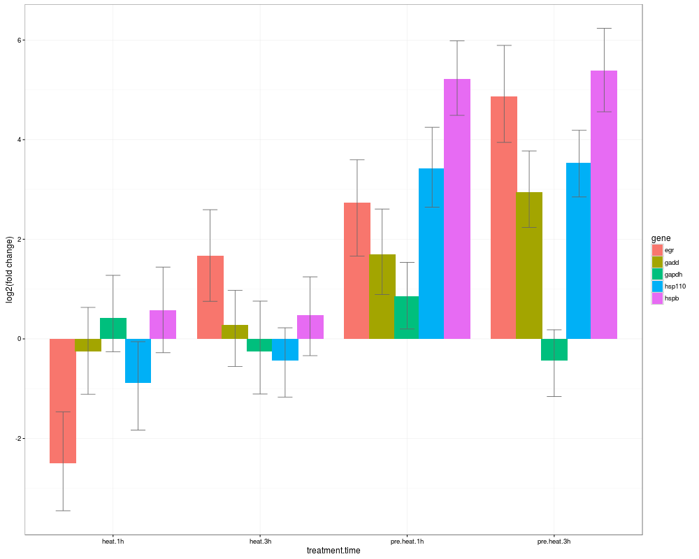
Summarizes and plots results of mcmc.qpcr function series.

Description

Calculates abundances of each gene across factor combinations; calculates pairwise differences between all factor combinations and their significances for each gene; plots results as bar or line graphs with credible intervals (ggplot2) NOTE: only works for experiments involving a single multi-level fixed factor or two fully crossed multi-level fixed factors.

Usage

HPDsummary(model, data, xgroup=NULL,genes = NA, relative = FALSE, 
log.base = 2, summ.plot = TRUE, ptype="z", ...)

Arguments

`model`	Model generated by mcmc.qpcr(),mcmc.qpcr.lognormal() or mcmc.qpcr.classic()
`data`	Dataset used to build the model (returned by cq2counts() or cq2log())
`xgroup`	The factor to form the x-axis of the plot. By default the first factor in the model will be used.
`genes`	A vector of gene names to summarize and plot. If left unspecified, all genes will be summarized.
`relative`	Whether to plot absolute transcript abundances (relative = FALSE) or fold- changes relative to the sample that is considered to be "global control" (relative = TRUE). The "global control" is the combination of factors that served as a reference during model fitting, either because it is alphanumerically first (that happens by default) or because it has been explicitly designated as such using relevel() function (see tutorial).
`log.base`	Base of the logarithm to use.
`summ.plot`	By default, the function generates a summary plot, which is a line-points-95% credible intervals plot of log(absolute abundances) with 'relative=FALSE' and a more typical bar graph of log(fold change relative to the control), again with 95% credible intervals, with 'relative=TRUE'. Specify 'summ.plot=FALSE' if you don't want the summary plot.
`ptype`	Which type of p-values to use. By default p-values based on the Bayesian z-score are used. Specify 'ptype="mcmc"' to output more conventional p-values based on MCMC sampling (these will be limited on the lower end by the size of MCMC sample).
`...`	Additional options for summaryPlot() function. Among those, 'x.order' can be a vector specifying the order of factor levels on the x-axis.

Value

A list of three items:

`summary`	Summary table containing calculated abundances, their SD and 95% credible limits
`geneWise`	A series of matrices listing pairwise differences between factor combinations (upper triangle) and corresponding p-values (lower triangle)
`ggPlot`	the ggplot2 object for plotting. See http://docs.ggplot2.org/0.9.2.1/theme.html for ways to modify it, such as add text, rotate labels, change fonts, etc.

Author(s)

Mikhail V. Matz, University of Texas at Austin <matz@utexas.edu>

References

Matz MV, Wright RM, Scott JG (2013) No Control Genes Required: Bayesian Analysis of qRT-PCR Data. PLoS ONE 8(8): e71448. doi:10.1371/journal.pone.0071448

Examples


data(beckham.data)
data(beckham.eff)

# analysing the first 5 genes 
# (to try it with all 10 genes, change the line below to gcol=4:13)
gcol=4:8 
ccol=1:3 # columns containing experimental conditions

# recalculating into molecule counts, reformatting
qs=cq2counts(data=beckham.data,genecols=gcol,
condcols=ccol,effic=beckham.eff,Cq1=37)

# creating a single factor, 'treatment.time', out of 'tr' and 'time'
qs$treatment.time=as.factor(paste(qs$tr,qs$time,sep="."))

# fitting a naive model
naive=mcmc.qpcr(
	fixed="treatment.time",
	data=qs,
	nitt=3000,burnin=2000 # remove this line in actual analysis!
)

#summary plot of inferred abundances
# s1=HPDsummary(model=naive,data=qs)

#summary plot of fold-changes relative to the global control
s0=HPDsummary(model=naive,data=qs,relative=TRUE)

# pairwise differences and their significances for each gene:
s0$geneWise

Results


R version 3.3.1 (2016-06-21) -- "Bug in Your Hair"
Copyright (C) 2016 The R Foundation for Statistical Computing
Platform: x86_64-pc-linux-gnu (64-bit)

R is free software and comes with ABSOLUTELY NO WARRANTY.
You are welcome to redistribute it under certain conditions.
Type 'license()' or 'licence()' for distribution details.

R is a collaborative project with many contributors.
Type 'contributors()' for more information and
'citation()' on how to cite R or R packages in publications.

Type 'demo()' for some demos, 'help()' for on-line help, or
'help.start()' for an HTML browser interface to help.
Type 'q()' to quit R.

> library(MCMC.qpcr)
Loading required package: MCMCglmm
Loading required package: Matrix
Loading required package: coda
Loading required package: ape
Loading required package: ggplot2
> png(filename="/home/ddbj/snapshot/RGM3/R_CC/result/MCMC.qpcr/HPDsummary.Rd_%03d_medium.png", width=480, height=480)
> ### Name: HPDsummary
> ### Title: Summarizes and plots results of mcmc.qpcr function series.
> ### Aliases: HPDsummary
> 
> ### ** Examples
> 
> 
> data(beckham.data)
> data(beckham.eff)
> 
> # analysing the first 5 genes 
> # (to try it with all 10 genes, change the line below to gcol=4:13)
> gcol=4:8 
> ccol=1:3 # columns containing experimental conditions
> 
> # recalculating into molecule counts, reformatting
> qs=cq2counts(data=beckham.data,genecols=gcol,
+ condcols=ccol,effic=beckham.eff,Cq1=37)
> 
> # creating a single factor, 'treatment.time', out of 'tr' and 'time'
> qs$treatment.time=as.factor(paste(qs$tr,qs$time,sep="."))
> 
> # fitting a naive model
> naive=mcmc.qpcr(
+ 	fixed="treatment.time",
+ 	data=qs,
+ 	nitt=3000,burnin=2000 # remove this line in actual analysis!
+ )
$PRIOR
$PRIOR$R
$PRIOR$R$V
     [,1] [,2] [,3] [,4] [,5]
[1,]    1    0    0    0    0
[2,]    0    1    0    0    0
[3,]    0    0    1    0    0
[4,]    0    0    0    1    0
[5,]    0    0    0    0    1

$PRIOR$R$nu
[1] 4.002


$PRIOR$G
$PRIOR$G$G1
$PRIOR$G$G1$V
[1] 1

$PRIOR$G$G1$nu
[1] 0




$FIXED
[1] "count~0+gene++gene:treatment.time"

$RANDOM
[1] "~sample"


                       MCMC iteration = 0

 Acceptance ratio for liability set 1 = 0.000385

 Acceptance ratio for liability set 2 = 0.000167

 Acceptance ratio for liability set 3 = 0.000143

 Acceptance ratio for liability set 4 = 0.000450

 Acceptance ratio for liability set 5 = 0.000462

                       MCMC iteration = 1000

 Acceptance ratio for liability set 1 = 0.122667

 Acceptance ratio for liability set 2 = 0.035238

 Acceptance ratio for liability set 3 = 0.008357

 Acceptance ratio for liability set 4 = 0.025250

 Acceptance ratio for liability set 5 = 0.032821

                       MCMC iteration = 2000

 Acceptance ratio for liability set 1 = 0.184846

 Acceptance ratio for liability set 2 = 0.057357

 Acceptance ratio for liability set 3 = 0.006000

 Acceptance ratio for liability set 4 = 0.037975

 Acceptance ratio for liability set 5 = 0.051436

                       MCMC iteration = 3000

 Acceptance ratio for liability set 1 = 0.201769

 Acceptance ratio for liability set 2 = 0.064619

 Acceptance ratio for liability set 3 = 0.006452

 Acceptance ratio for liability set 4 = 0.041425

 Acceptance ratio for liability set 5 = 0.058154
> 
> #summary plot of inferred abundances
> # s1=HPDsummary(model=naive,data=qs)
> 
> #summary plot of fold-changes relative to the global control
> s0=HPDsummary(model=naive,data=qs,relative=TRUE)
> 
> # pairwise differences and their significances for each gene:
> s0$geneWise
$egr
             difference
pvalue          control.0h       heat.1h      heat.3h pre.heat.1h pre.heat.3h
  control.0h            NA -2.327858e+00 1.854407e+00 2.833691585    4.957891
  heat.1h     4.483250e-05            NA 4.182265e+00 5.161549620    7.285749
  heat.3h     2.281443e-03  2.926881e-11           NA 0.979284274    3.103483
  pre.heat.1h 5.523180e-06  1.554312e-15 1.185160e-01          NA    2.124199
  pre.heat.3h 4.440892e-16  0.000000e+00 5.571835e-07 0.001090859          NA

$gadd
             difference
pvalue          control.0h       heat.1h      heat.3h pre.heat.1h pre.heat.3h
  control.0h            NA -6.020411e-02 3.237088e-01  1.78375467    3.010255
  heat.1h     8.922235e-01            NA 3.839129e-01  1.84395878    3.070459
  heat.3h     4.788135e-01  4.370183e-01           NA  1.46004590    2.686547
  pre.heat.1h 3.470603e-05  1.349279e-04 9.962803e-04          NA    1.226501
  pre.heat.3h 1.390690e-08  1.225225e-08 4.316809e-07  0.02109475          NA

$gapdh
             difference
pvalue        control.0h    heat.1h     heat.3h pre.heat.1h pre.heat.3h
  control.0h          NA 0.53610325 -0.13107656  0.96882842  -0.3005155
  heat.1h     0.25878269         NA -0.66717981  0.43272517  -0.8366187
  heat.3h     0.80256669 0.18697540          NA  1.09990498  -0.1694389
  pre.heat.1h 0.04614115 0.38561023  0.02893827          NA  -1.2693439
  pre.heat.3h 0.54869907 0.09934648  0.73028210  0.01586384          NA

$hsp110
             difference
pvalue          control.0h    heat.1h       heat.3h pre.heat.1h pre.heat.3h
  control.0h            NA -0.6720907 -3.867444e-01   3.5366114   3.5657399
  heat.1h     1.733211e-01         NA  2.853463e-01   4.2087021   4.2378306
  heat.3h     4.526113e-01  0.5877312            NA   3.9233558   3.9524843
  pre.heat.1h 1.028644e-11  0.0000000  1.481038e-12          NA   0.0291285
  pre.heat.3h 6.534062e-11  0.0000000  4.543921e-12   0.9593276          NA

$hspb
             difference
pvalue        control.0h   heat.1h       heat.3h pre.heat.1h pre.heat.3h
  control.0h          NA 0.6792636  4.657386e-01   5.3644282   5.4736501
  heat.1h      0.1160298        NA -2.135250e-01   4.6851646   4.7943865
  heat.3h      0.4060847 0.7056827            NA   4.8986896   5.0079115
  pre.heat.1h  0.0000000 0.0000000  2.220446e-16          NA   0.1092219
  pre.heat.3h  0.0000000 0.0000000  0.000000e+00   0.8411291          NA

> 
> 
> 
> 
> 
> 
> dev.off()
null device 
          1 
>