Supported by Dr. Osamu Ogasawara and  . . |
|
Last data update: 2014.03.03 |
Bayesian analysis of qRT-PCR dataDescriptionThis package implements generalized linear mixed model analysis of qRT-PCR data so that the increase of variance towards higher Ct values is properly dealt with, and the lack of amplification is informative (function mcmc.qpcr). Sample-loading effects, gene-specific variances, and responses of all genes to each factor combination are all jointly estimated within a single model. The control genes can be specified as priors, with adjustable degree of expected stability. The analysis also works well without any control gene specifications. For higher-abundance datasets, a lognormal model is implemented that does not require Cq to counts conversion (function mcmc.qpcr.lognormal). For higher-abundance datasets datasets in which the quality and/or quantity of RNA samples varies systematically (rather than randomly) across conditions, the analysis based on multigene normalization is implemented (function mcmc.qpcr.classic). The package includes several functions for plotting the results and calculating statistical significance (HPDplot, HPDplotBygene, HPDplotBygeneBygroup). The detailed step-by-step tutorial is here: http://www.bio.utexas.edu/research/matz_lab/matzlab/Methods_files/mcmc.qpcr.tutorial.pdf. Details
Author(s)Mikhail V. Matz, University of Texas at Austin <matz@utexas.edu> ReferencesMatz MV, Wright RM, Scott JG (2013) No Control Genes Required: Bayesian Analysis of qRT-PCR Data. PLoS ONE 8(8): e71448. doi:10.1371/journal.pone.0071448 Examplesdata(beckham.data) data(beckham.eff) # analysing the first 5 genes # (to try it with all 10 genes, change the line below to gcol=4:13) gcol=4:8 ccol=1:3 # columns containing experimental conditions # recalculating into molecule counts, reformatting qs=cq2counts(data=beckham.data,genecols=gcol, condcols=ccol,effic=beckham.eff,Cq1=37) # creating a single factor, 'treatment.time', out of 'tr' and 'time' qs$treatment.time=as.factor(paste(qs$tr,qs$time,sep=".")) # fitting a naive model naive=mcmc.qpcr( fixed="treatment.time", data=qs, nitt=3000,burnin=2000 # remove this line in actual analysis! ) #summary plot of inferred abundances #s1=HPDsummary(model=naive,data=qs) #summary plot of fold-changes relative to the global control s0=HPDsummary(model=naive,data=qs,relative=TRUE) # pairwise differences and their significances for each gene: s0$geneWise Results
R version 3.3.1 (2016-06-21) -- "Bug in Your Hair"
Copyright (C) 2016 The R Foundation for Statistical Computing
Platform: x86_64-pc-linux-gnu (64-bit)
R is free software and comes with ABSOLUTELY NO WARRANTY.
You are welcome to redistribute it under certain conditions.
Type 'license()' or 'licence()' for distribution details.
R is a collaborative project with many contributors.
Type 'contributors()' for more information and
'citation()' on how to cite R or R packages in publications.
Type 'demo()' for some demos, 'help()' for on-line help, or
'help.start()' for an HTML browser interface to help.
Type 'q()' to quit R.
> library(MCMC.qpcr)
Loading required package: MCMCglmm
Loading required package: Matrix
Loading required package: coda
Loading required package: ape
Loading required package: ggplot2
> png(filename="/home/ddbj/snapshot/RGM3/R_CC/result/MCMC.qpcr/MCMC.qpcr-package.Rd_%03d_medium.png", width=480, height=480)
> ### Name: MCMC.qpcr-package
> ### Title: Bayesian analysis of qRT-PCR data
> ### Aliases: MCMC.qpcr
> ### Keywords: package
>
> ### ** Examples
>
>
> data(beckham.data)
> data(beckham.eff)
>
> # analysing the first 5 genes
> # (to try it with all 10 genes, change the line below to gcol=4:13)
> gcol=4:8
> ccol=1:3 # columns containing experimental conditions
>
> # recalculating into molecule counts, reformatting
> qs=cq2counts(data=beckham.data,genecols=gcol,
+ condcols=ccol,effic=beckham.eff,Cq1=37)
>
> # creating a single factor, 'treatment.time', out of 'tr' and 'time'
> qs$treatment.time=as.factor(paste(qs$tr,qs$time,sep="."))
>
> # fitting a naive model
> naive=mcmc.qpcr(
+ fixed="treatment.time",
+ data=qs,
+ nitt=3000,burnin=2000 # remove this line in actual analysis!
+ )
$PRIOR
$PRIOR$R
$PRIOR$R$V
[,1] [,2] [,3] [,4] [,5]
[1,] 1 0 0 0 0
[2,] 0 1 0 0 0
[3,] 0 0 1 0 0
[4,] 0 0 0 1 0
[5,] 0 0 0 0 1
$PRIOR$R$nu
[1] 4.002
$PRIOR$G
$PRIOR$G$G1
$PRIOR$G$G1$V
[1] 1
$PRIOR$G$G1$nu
[1] 0
$FIXED
[1] "count~0+gene++gene:treatment.time"
$RANDOM
[1] "~sample"
MCMC iteration = 0
Acceptance ratio for liability set 1 = 0.000333
Acceptance ratio for liability set 2 = 0.000405
Acceptance ratio for liability set 3 = 0.000190
Acceptance ratio for liability set 4 = 0.000450
Acceptance ratio for liability set 5 = 0.000487
MCMC iteration = 1000
Acceptance ratio for liability set 1 = 0.119000
Acceptance ratio for liability set 2 = 0.036976
Acceptance ratio for liability set 3 = 0.008071
Acceptance ratio for liability set 4 = 0.027450
Acceptance ratio for liability set 5 = 0.034128
MCMC iteration = 2000
Acceptance ratio for liability set 1 = 0.179949
Acceptance ratio for liability set 2 = 0.056714
Acceptance ratio for liability set 3 = 0.005976
Acceptance ratio for liability set 4 = 0.039575
Acceptance ratio for liability set 5 = 0.048487
MCMC iteration = 3000
Acceptance ratio for liability set 1 = 0.195769
Acceptance ratio for liability set 2 = 0.067738
Acceptance ratio for liability set 3 = 0.006310
Acceptance ratio for liability set 4 = 0.046325
Acceptance ratio for liability set 5 = 0.051744
>
> #summary plot of inferred abundances
> #s1=HPDsummary(model=naive,data=qs)
>
> #summary plot of fold-changes relative to the global control
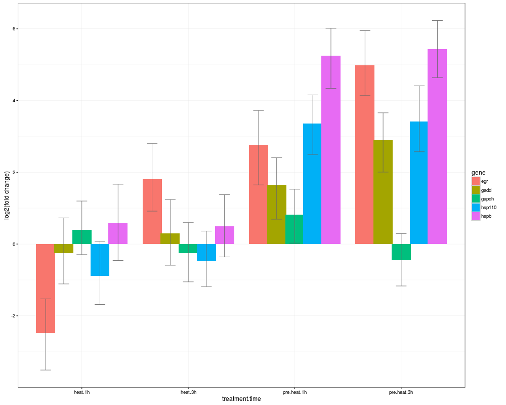
> s0=HPDsummary(model=naive,data=qs,relative=TRUE)
>
> # pairwise differences and their significances for each gene:
> s0$geneWise
$egr
difference
pvalue control.0h heat.1h heat.3h pre.heat.1h pre.heat.3h
control.0h NA -2.385451e+00 1.914256e+00 2.8673035260 4.920286
heat.1h 1.267956e-04 NA 4.299707e+00 5.2527545241 7.305737
heat.3h 1.161913e-03 3.865797e-12 NA 0.9530475908 3.006030
pre.heat.1h 9.730431e-06 0.000000e+00 1.543370e-01 NA 2.052983
pre.heat.3h 2.442491e-15 0.000000e+00 2.190127e-06 0.0001584982 NA
$gadd
difference
pvalue control.0h heat.1h heat.3h pre.heat.1h pre.heat.3h
control.0h NA -1.341062e-01 4.185646e-01 1.77673585 2.988818
heat.1h 8.048195e-01 NA 5.526708e-01 1.91084207 3.122924
heat.3h 4.368305e-01 3.252171e-01 NA 1.35817129 2.570253
pre.heat.1h 1.125570e-03 1.304911e-04 1.116688e-02 NA 1.212082
pre.heat.3h 1.922578e-10 7.859209e-10 4.568188e-06 0.02782503 NA
$gapdh
difference
pvalue control.0h heat.1h heat.3h pre.heat.1h pre.heat.3h
control.0h NA 0.61378012 -0.0775170 0.999518793 -0.3176251
heat.1h 0.2427278 NA -0.6912971 0.385738669 -0.9314053
heat.3h 0.8757274 0.20737156 NA 1.077035790 -0.2401081
pre.heat.1h 0.0438083 0.41548421 0.0295172 NA -1.3171439
pre.heat.3h 0.5108244 0.07445655 0.6181846 0.003958731 NA
$hsp110
difference
pvalue control.0h heat.1h heat.3h pre.heat.1h pre.heat.3h
control.0h NA -7.920780e-01 -3.004749e-01 3.5355989 3.533248317
heat.1h 2.119180e-01 NA 4.916031e-01 4.3276769 4.325326296
heat.3h 6.113113e-01 4.162080e-01 NA 3.8360738 3.833723193
pre.heat.1h 6.539645e-09 0.000000e+00 3.392842e-12 NA -0.002350614
pre.heat.3h 3.195888e-12 8.881784e-15 1.663336e-11 0.9962737 NA
$hspb
difference
pvalue control.0h heat.1h heat.3h pre.heat.1h pre.heat.3h
control.0h NA 7.545748e-01 0.7274476 5.4322019 5.50236639
heat.1h 0.2092323 NA -0.0271272 4.6776271 4.74779155
heat.3h 0.1822699 9.658182e-01 NA 4.7047543 4.77491875
pre.heat.1h 0.0000000 9.547918e-15 0.0000000 NA 0.07016448
pre.heat.3h 0.0000000 0.000000e+00 0.0000000 0.9011167 NA
>
>
>
>
>
>
> dev.off()
null device
1
>
|