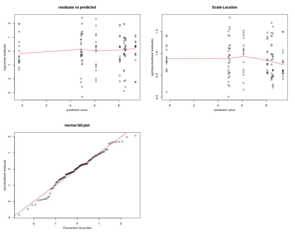
Plots three diagnostic plots to check the validity of the assumptions of linear model analysis.

Description

Predicted vs observed plot tests for linearity, Scale-location plot tests for homoscedasticity, and Normal QQ plot tests for normality of the residuals.

Usage

diagnostic.mcmc(model, ...)

Arguments

Value

A plot with three panels.

Author(s)

Mikhail V. Matz, UT Austin <matz@utexas.edu>

References

Matz MV, Wright RM, Scott JG (2013) No Control Genes Required: Bayesian Analysis of qRT-PCR Data. PLoS ONE 8(8): e71448. doi:10.1371/journal.pone.0071448

Examples

# loading Cq data and amplification efficiencies
data(coral.stress) 
data(amp.eff) 
# extracting a subset of data 
cs.short=subset(coral.stress, timepoint=="one")

genecolumns=c(5,6,16,17) # specifying columns corresponding to genes of interest
conditions=c(1:4) # specifying columns containing factors  

# calculating molecule counts and reformatting:
dd=cq2counts(data=cs.short,genecols=genecolumns,
condcols=conditions,effic=amp.eff,Cq1=37) 

# fitting the model
mm=mcmc.qpcr(
	fixed="condition",
	data=dd,
	controls=c("nd5","rpl11"),
	pr=TRUE,pl=TRUE, # these flags are necessary for diagnostics
	nitt=4000 # remove this line when analyzing real data!
)
diagnostic.mcmc(mm)

Results

R version 3.3.1 (2016-06-21) -- "Bug in Your Hair"
Copyright (C) 2016 The R Foundation for Statistical Computing
Platform: x86_64-pc-linux-gnu (64-bit)

R is free software and comes with ABSOLUTELY NO WARRANTY.
You are welcome to redistribute it under certain conditions.
Type 'license()' or 'licence()' for distribution details.

R is a collaborative project with many contributors.
Type 'contributors()' for more information and
'citation()' on how to cite R or R packages in publications.

Type 'demo()' for some demos, 'help()' for on-line help, or
'help.start()' for an HTML browser interface to help.
Type 'q()' to quit R.

> library(MCMC.qpcr)
Loading required package: MCMCglmm
Loading required package: Matrix
Loading required package: coda
Loading required package: ape
Loading required package: ggplot2
> png(filename="/home/ddbj/snapshot/RGM3/R_CC/result/MCMC.qpcr/diagnostic.mcmc.Rd_%03d_medium.png", width=480, height=480)
> ### Name: diagnostic.mcmc
> ### Title: Plots three diagnostic plots to check the validity of the
> ###   assumptions of linear model analysis.
> ### Aliases: diagnostic.mcmc
> 
> ### ** Examples
> 
> 
> # loading Cq data and amplification efficiencies
> data(coral.stress) 
> data(amp.eff) 
> # extracting a subset of data 
> cs.short=subset(coral.stress, timepoint=="one")
> 
> genecolumns=c(5,6,16,17) # specifying columns corresponding to genes of interest
> conditions=c(1:4) # specifying columns containing factors  
> 
> # calculating molecule counts and reformatting:
> dd=cq2counts(data=cs.short,genecols=genecolumns,
+ condcols=conditions,effic=amp.eff,Cq1=37) 
> 
> # fitting the model
> mm=mcmc.qpcr(
+ 	fixed="condition",
+ 	data=dd,
+ 	controls=c("nd5","rpl11"),
+ 	pr=TRUE,pl=TRUE, # these flags are necessary for diagnostics
+ 	nitt=4000 # remove this line when analyzing real data!
+ )
$PRIOR
$PRIOR$B
$PRIOR$B$mu
[1] 0 0 0 0 0 0 0 0

$PRIOR$B$V
      [,1]  [,2]  [,3]  [,4]  [,5]  [,6]      [,7]      [,8]
[1,] 1e+08 0e+00 0e+00 0e+00 0e+00 0e+00 0.0000000 0.0000000
[2,] 0e+00 1e+08 0e+00 0e+00 0e+00 0e+00 0.0000000 0.0000000
[3,] 0e+00 0e+00 1e+08 0e+00 0e+00 0e+00 0.0000000 0.0000000
[4,] 0e+00 0e+00 0e+00 1e+08 0e+00 0e+00 0.0000000 0.0000000
[5,] 0e+00 0e+00 0e+00 0e+00 1e+08 0e+00 0.0000000 0.0000000
[6,] 0e+00 0e+00 0e+00 0e+00 0e+00 1e+08 0.0000000 0.0000000
[7,] 0e+00 0e+00 0e+00 0e+00 0e+00 0e+00 0.3663091 0.0000000
[8,] 0e+00 0e+00 0e+00 0e+00 0e+00 0e+00 0.0000000 0.3663091


$PRIOR$R
$PRIOR$R$V
     [,1] [,2] [,3] [,4]
[1,]    1    0    0    0
[2,]    0    1    0    0
[3,]    0    0    1    0
[4,]    0    0    0    1

$PRIOR$R$nu
[1] 3.002


$PRIOR$G
$PRIOR$G$G1
$PRIOR$G$G1$V
[1] 1

$PRIOR$G$G1$nu
[1] 0




$FIXED
[1] "count~0+gene++gene:condition"

$RANDOM
[1] "~sample"


                       MCMC iteration = 0

 Acceptance ratio for liability set 1 = 0.000500

 Acceptance ratio for liability set 2 = 0.000516

 Acceptance ratio for liability set 3 = 0.000194

 Acceptance ratio for liability set 4 = 0.000313

                       MCMC iteration = 1000

 Acceptance ratio for liability set 1 = 0.100469

 Acceptance ratio for liability set 2 = 0.379032

 Acceptance ratio for liability set 3 = 0.308935

 Acceptance ratio for liability set 4 = 0.115406

                       MCMC iteration = 2000

 Acceptance ratio for liability set 1 = 0.158500

 Acceptance ratio for liability set 2 = 0.422839

 Acceptance ratio for liability set 3 = 0.358935

 Acceptance ratio for liability set 4 = 0.173063

                       MCMC iteration = 3000

 Acceptance ratio for liability set 1 = 0.185656

 Acceptance ratio for liability set 2 = 0.432645

 Acceptance ratio for liability set 3 = 0.366387

 Acceptance ratio for liability set 4 = 0.204250

                       MCMC iteration = 4000

 Acceptance ratio for liability set 1 = 0.200375

 Acceptance ratio for liability set 2 = 0.439484

 Acceptance ratio for liability set 3 = 0.338484

 Acceptance ratio for liability set 4 = 0.231406
> diagnostic.mcmc(mm)
> 
> 
> 
> 
> 
> 
> dev.off()
null device 
          1 
>