R Graphical Manual

Browse All

Last data update: 2014.03.03

R: Extracts qPCR model predictions

getNormalizedData

R Documentation

Extracts qPCR model predictions

Description

Generates a table of model-derived log2-transformed transcript abundances without global sample effects (i.e., corresponding to efficiency-corrected and normalized qPCR data)

Usage

getNormalizedData(model, data, controls=NULL)

Arguments

`model`	qPCR model: the output of mcmc.qpcr or mcmc.qpcr.lognormal function fitted with two additional options: random="sample", pr=TRUE . These options do not change the inferences of main effects but make it possible to retain among-sample variation of expression for each gene while still subtracting the global sample effects (i.e., perform "normalization")
`data`	The dataset that was analysed to generate the model (output of cq2counts or cq2log functions)
`controls`	List of control genes; required if the mcmc.qpcr model was fit with the option normalize=TRUE

Value

The function returns a list of two data frames. The first one, normData, is the model-predicted log2-transformed transcript abundances table. It has one column per gene and one row per sample. The second data frame, conditions, is a table of experimental conditions corresponding to the normData table.

Author(s)

Mikhail V. Matz, University of Texas at Austin <matz@utexas.edu>

References

Matz MV, Wright RM, Scott JG (2013) No Control Genes Required: Bayesian Analysis of qRT-PCR Data. PLoS ONE 8(8): e71448. doi:10.1371/journal.pone.0071448

Examples

library(MCMC.qpcr)

# loading Cq data and amplification efficiencies
data(coral.stress) 
data(amp.eff) 

genecolumns=c(5,6,16,17) # specifying columns corresponding to genes of interest
conditions=c(1:4) # specifying columns containing factors  

# calculating molecule counts and reformatting:
dd=cq2counts(data=coral.stress,genecols=genecolumns,
condcols=conditions,effic=amp.eff,Cq1=37) 

# fitting the model (must include random="sample", pr=TRUE options)
mm=mcmc.qpcr(
	fixed="condition",
	data=dd,
	controls=c("nd5","rpl11"),
	nitt=4000,
	pr=TRUE,
	random="sample"
)

# extracting model predictions
pp=getNormalizedData(mm,dd)

# here is the normalized data:
pp$normData

# and here are the corresponding conditions:
pp$conditions

# putting them together for plotting:
ppcombo=cbind(stack(pp$normData),rep(pp$conditions))
names(ppcombo)[1:2]=c("expression","gene")

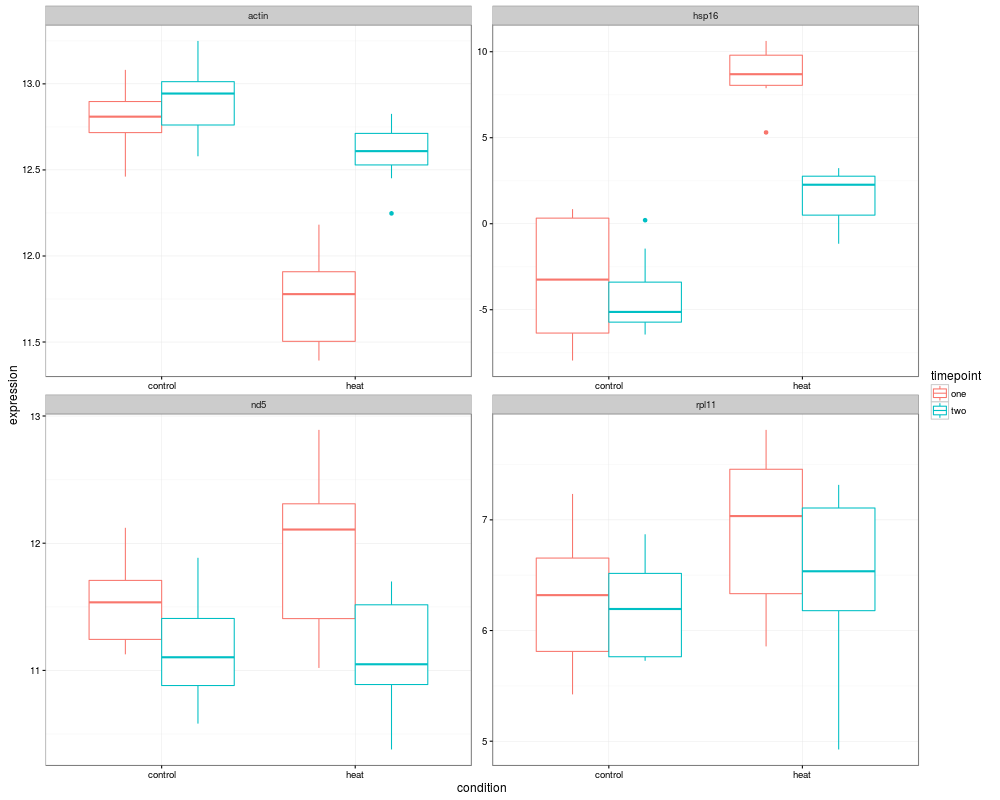
# plotting boxplots of normalized data:
ggplot(ppcombo,aes(condition,expression,colour=timepoint))+
	geom_boxplot()+
	facet_wrap(~gene,scales="free")+
	theme_bw()

Results


R version 3.3.1 (2016-06-21) -- "Bug in Your Hair"
Copyright (C) 2016 The R Foundation for Statistical Computing
Platform: x86_64-pc-linux-gnu (64-bit)

R is free software and comes with ABSOLUTELY NO WARRANTY.
You are welcome to redistribute it under certain conditions.
Type 'license()' or 'licence()' for distribution details.

R is a collaborative project with many contributors.
Type 'contributors()' for more information and
'citation()' on how to cite R or R packages in publications.

Type 'demo()' for some demos, 'help()' for on-line help, or
'help.start()' for an HTML browser interface to help.
Type 'q()' to quit R.

> library(MCMC.qpcr)
Loading required package: MCMCglmm
Loading required package: Matrix
Loading required package: coda
Loading required package: ape
Loading required package: ggplot2
> png(filename="/home/ddbj/snapshot/RGM3/R_CC/result/MCMC.qpcr/getNormalizedData.Rd_%03d_medium.png", width=480, height=480)
> ### Name: getNormalizedData
> ### Title: Extracts qPCR model predictions
> ### Aliases: getNormalizedData
> 
> ### ** Examples
> 
> library(MCMC.qpcr)
> 
> # loading Cq data and amplification efficiencies
> data(coral.stress) 
> data(amp.eff) 
> 
> genecolumns=c(5,6,16,17) # specifying columns corresponding to genes of interest
> conditions=c(1:4) # specifying columns containing factors  
> 
> # calculating molecule counts and reformatting:
> dd=cq2counts(data=coral.stress,genecols=genecolumns,
+ condcols=conditions,effic=amp.eff,Cq1=37) 
> 
> # fitting the model (must include random="sample", pr=TRUE options)
> mm=mcmc.qpcr(
+ 	fixed="condition",
+ 	data=dd,
+ 	controls=c("nd5","rpl11"),
+ 	nitt=4000,
+ 	pr=TRUE,
+ 	random="sample"
+ )
$PRIOR
$PRIOR$B
$PRIOR$B$mu
[1] 0 0 0 0 0 0 0 0

$PRIOR$B$V
      [,1]  [,2]  [,3]  [,4]  [,5]  [,6]      [,7]      [,8]
[1,] 1e+08 0e+00 0e+00 0e+00 0e+00 0e+00 0.0000000 0.0000000
[2,] 0e+00 1e+08 0e+00 0e+00 0e+00 0e+00 0.0000000 0.0000000
[3,] 0e+00 0e+00 1e+08 0e+00 0e+00 0e+00 0.0000000 0.0000000
[4,] 0e+00 0e+00 0e+00 1e+08 0e+00 0e+00 0.0000000 0.0000000
[5,] 0e+00 0e+00 0e+00 0e+00 1e+08 0e+00 0.0000000 0.0000000
[6,] 0e+00 0e+00 0e+00 0e+00 0e+00 1e+08 0.0000000 0.0000000
[7,] 0e+00 0e+00 0e+00 0e+00 0e+00 0e+00 0.3663091 0.0000000
[8,] 0e+00 0e+00 0e+00 0e+00 0e+00 0e+00 0.0000000 0.3663091


$PRIOR$R
$PRIOR$R$V
     [,1] [,2] [,3] [,4]
[1,]    1    0    0    0
[2,]    0    1    0    0
[3,]    0    0    1    0
[4,]    0    0    0    1

$PRIOR$R$nu
[1] 3.002


$PRIOR$G
$PRIOR$G$G1
$PRIOR$G$G1$V
[1] 1

$PRIOR$G$G1$nu
[1] 0


$PRIOR$G$G2
$PRIOR$G$G2$V
     [,1] [,2] [,3] [,4]
[1,]    1    0    0    0
[2,]    0    1    0    0
[3,]    0    0    1    0
[4,]    0    0    0    1

$PRIOR$G$G2$nu
[1] 0




$FIXED
[1] "count~0+gene++gene:condition"

$RANDOM
[1] "~sample+idh(gene):sample"


                       MCMC iteration = 0

 Acceptance ratio for liability set 1 = 0.000266

 Acceptance ratio for liability set 2 = 0.000635

 Acceptance ratio for liability set 3 = 0.000365

 Acceptance ratio for liability set 4 = 0.000203

                       MCMC iteration = 1000

 Acceptance ratio for liability set 1 = 0.125984

 Acceptance ratio for liability set 2 = 0.311238

 Acceptance ratio for liability set 3 = 0.303825

 Acceptance ratio for liability set 4 = 0.156094

                       MCMC iteration = 2000

 Acceptance ratio for liability set 1 = 0.188672

 Acceptance ratio for liability set 2 = 0.333730

 Acceptance ratio for liability set 3 = 0.336190

 Acceptance ratio for liability set 4 = 0.225453

                       MCMC iteration = 3000

 Acceptance ratio for liability set 1 = 0.221359

 Acceptance ratio for liability set 2 = 0.337667

 Acceptance ratio for liability set 3 = 0.339937

 Acceptance ratio for liability set 4 = 0.248109

                       MCMC iteration = 4000

 Acceptance ratio for liability set 1 = 0.240172

 Acceptance ratio for liability set 2 = 0.318571

 Acceptance ratio for liability set 3 = 0.337587

 Acceptance ratio for liability set 4 = 0.264609
> 
> # extracting model predictions
> pp=getNormalizedData(mm,dd)
> 
> # here is the normalized data:
> pp$normData
         hsp16    actin      nd5    rpl11
1  -3.47795277 12.87418 11.28497 7.297597
2   8.02000728 12.12638 10.94048 7.733618
3  -3.19970389 12.71495 12.09723 7.190185
4   8.16632198 12.10252 11.25693 7.123951
5   1.19866768 12.99997 12.27613 5.611415
6  10.79611433 11.68718 12.52507 7.802915
7  -3.43122561 13.15043 11.76310 5.637348
8   7.84303179 11.97914 12.21349 7.527204
9  -5.84196734 12.89903 11.58675 6.606744
10  9.92617984 11.78224 13.17928 6.552712
11 -5.48344313 13.07968 11.54714 5.929344
12  5.41325748 11.94335 12.49211 6.398555
13  0.73702153 12.80468 11.22311 6.275081
14 10.10344639 12.10784 11.56307 5.954321
15  0.35690004 12.98063 11.38833 6.650236
16  9.32905374 11.80912 12.27635 7.319336
17 -7.87154891 13.16756 10.41543 6.645269
18  3.02292658 12.51073 10.63188 7.074402
19 -5.00036847 13.08979 11.06974 6.448193
20  2.92466513 12.41626 10.81831 6.977519
21 -0.01102747 13.05266 11.52856 5.736194
22  2.67675379 12.17872 11.45970 6.604527
23 -0.98393605 13.00210 10.83387 7.054781
24  0.29151508 12.51993 10.13565 7.090342
25 -3.34059262 12.82451 11.42666 6.350209
26  0.23181204 12.35630 11.66513 4.756375
27 -5.34260503 12.81584 11.94863 6.034343
28  1.79189767 12.36196 11.45611 6.134166
29 -5.91553808 13.04340 10.93324 6.522172
30  2.50818704 12.46471 10.89419 6.386004
31 -4.56205184 12.96699 11.61048 5.931506
32 -0.55396734 12.51844 10.87108 6.130582
> 
> # and here are the corresponding conditions:
> pp$conditions
   individual condition timepoint
1          s1   control       one
2          s1      heat       one
3          s2   control       one
4          s2      heat       one
5          s4   control       one
6          s4      heat       one
7          s5   control       one
8          s5      heat       one
9          s8   control       one
10         s8      heat       one
11        s12   control       one
12        s12      heat       one
13        s13   control       one
14        s13      heat       one
15        s15   control       one
16        s15      heat       one
17         s1   control       two
18         s1      heat       two
19         s2   control       two
20         s2      heat       two
21         s4   control       two
22         s4      heat       two
23         s5   control       two
24         s5      heat       two
25         s8   control       two
26         s8      heat       two
27        s12   control       two
28        s12      heat       two
29        s13   control       two
30        s13      heat       two
31        s15   control       two
32        s15      heat       two
> 
> # putting them together for plotting:
> ppcombo=cbind(stack(pp$normData),rep(pp$conditions))
> names(ppcombo)[1:2]=c("expression","gene")
> 
> # plotting boxplots of normalized data:
> ggplot(ppcombo,aes(condition,expression,colour=timepoint))+
+ 	geom_boxplot()+
+ 	facet_wrap(~gene,scales="free")+
+ 	theme_bw()
> 
> 
> 
> 
> 
> dev.off()
null device 
          1 
>