R Graphical Manual

Browse All

Last data update: 2014.03.03

R: Analyzes qRT-PCR data using generalized linear mixed model

mcmc.qpcr

R Documentation

Analyzes qRT-PCR data using generalized linear mixed model

Description

Wrapper function for MCMCglmm by Jarrod Hadfield, designed for qRT-PCR data analysis.

Usage

mcmc.qpcr(fixed=NULL, globalFixed=NULL, random = NULL, globalRandom=NULL, data, 
controls = NULL, normalize=FALSE, include = NULL, m.fix = 1.2, v.fix = NULL, 
geneSpecRes=TRUE, Covar=FALSE, vprior="uninf", ...)

Arguments

`fixed`	desired combination of fixed effects, as a text string. Do not use "*" symbol, list it fully, such as: 'factor1+factor2+factor1:factor2'.
`globalFixed`	Vector of fixed covariates (categorical or continuous) that are expected to affect all genes in the sample in the same way. These would be typically related to quality and/or quantity of RNA, such as RIN value.
`random`	A vector of names for gene-specific scalar random effects, such as 'c("effect1","effect2")'.
`globalRandom`	Random covariates (categorical only) affecting all genes, similar to globalFixed.
`data`	output of the cq2counts() function
`controls`	Vector of control gene names. These will be pushed to the back of the gene list during model fitting, in the reverse order. Controls are NOT NECESSARY for the analysis.
`normalize`	If controls are specified, requiring 'normalize=TRUE' will perform "soft normalization": the geometric mean of control genes will be used to infer global effects (common to all genes) across conditions; these will be subtracted when summarizing the data with HPDsummary(). Use this option when template abundances are correlated with conditions. Note that this is different from normalizing data within each sample, as per Vandesompele et al 2002; this would be "hard normalization" (use mcmc.qpcr.classic() if you want it).
`include`	How many of the control genes ('controls') to actually incorporate as priors during model fitting. If left unspecified, all the 'controls' will be used. If 'include=0', the model will be fitted without using any of the control genes as priors. If 'include' equals some number less than the number of 'controls', only the first 'include' of them will be used as priors. In all these cases, the 'controls' will appear in the same order in the output, in the end of the gene list rather than according to their alphabetical position among other genes. This is useful when visually comparing the results of models fitted with different number of control genes, using HPDplot and HPDpoints functions.
`m.fix`	Allowed average fold-change of the control genes in response to any fixed factor combination.
`v.fix`	Allowed residual fold-change deviation of the control genes. Applies to the residual variation term.
`geneSpecRes`	Whether the model should include gene-specific residuals. Keep it TRUE unless the model fails to converge.
`Covar`	Whether the random effects should be fitted with covariances. This option might require setting vprior="iw" or vprior="iw01" (see below)
`vprior`	The default prior is an uninformative inverse Wishart with assumed variance (V) at 1 and the degree of belief parameter (nu) at 0. With 'prior="iw"' and 'prior="iw01"' nu is equal [number of genes]-0.998, resulting in a weakly informative prior that is commonly used in this type of inference. vprior="iw" will assume large prior variance (1), vprior="iw01" will assume small prior variance (0.1).
`...`	other options for MCMCglmm function, such as nitt (number of iterations), thin (tinning interval), and burnin (number of initial iterations to disregard). For a more precise inference specify 'nitt=45000, thin=20, burnin=5000'. See MCMCglmm documentation for more details.

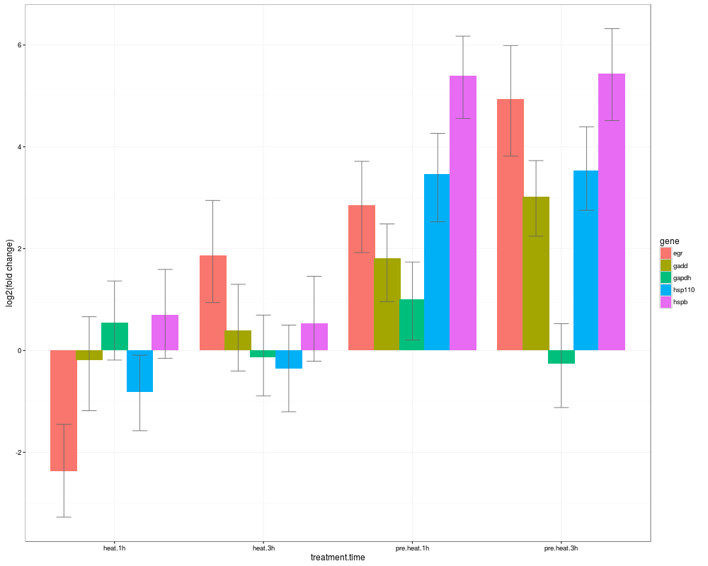
Details

This function constructs priors and runs an MCMC chain to fit a Poisson-lognormal generalized linear mixed model to the counts data.

The fixed effects for the model by default assume a gene-specific intercept, and gene-specific effect for each of the listed fixed factors.

The user-specified random effects are all assumed to be gene-specific with no covariances.

There is also a universal random factor: the scalar random effect of sample, which accounts for the unequal template loading.

Residual variances are assumed to be gene-specific with no covariances, with weakly informative inverse Wishart prior (variance=1, nu=[number of genes]-0.998).

The priors for fixed effects are diffuse gaussians with a mean at 0 and very large variances (1e+8), except for control genes, for which the prior variances are defined by the m.fix parameter. For the gene-specific random effects and residual variation, non-informative priors are used to achieve results equivalent to ML estimation. For control genes, when v.fix parameter is specified, it will be used to restrict residial variance.

Both m.fix and v.fix parameters should be specified as allowed average fold-change, so the lowest they can go is 1 (no variation).

All control genes share the same m.fix and v.fix parameters.

Value

An MCMCglmm object. HPDsummary() function within this package summaizes these data, calculates all gene-wise credible intervals and p-values, and plots the results either as line-point-whiskers graph or a bar-whiskers graph using ggplot2 functions.

HPDsummary() only works for experiments with a single multilevel factor or two fully crossed multilevel factors. Use finctions HPDplot(), HPDplotBygene() and HPDplotBygeneBygroup() to summarize and plot more complicated designs.

For more useful operations on MCMCglmm objects, such as posterior.mode(), HPDinterval(), and plot(), see documentation for MCMCglmm package.

Author(s)

Mikhail V. Matz, University of Texas at Austin <matz@utexas.edu>

References

Matz MV, Wright RM, Scott JG (2013) No Control Genes Required: Bayesian Analysis of qRT-PCR Data. PLoS ONE 8(8): e71448. doi:10.1371/journal.pone.0071448

Examples


data(beckham.data)
data(beckham.eff)

# analysing the first 5 genes 
# (to try it with all 10 genes, change the line below to gcol=4:13)
gcol=4:8 
ccol=1:3 # columns containing experimental conditions

# recalculating into molecule counts, reformatting
qs=cq2counts(data=beckham.data,genecols=gcol,
condcols=ccol,effic=beckham.eff,Cq1=37)

# creating a single factor, 'treatment.time', out of 'tr' and 'time'
qs$treatment.time=as.factor(paste(qs$tr,qs$time,sep="."))

# fitting a naive model
naive=mcmc.qpcr(
	fixed="treatment.time",
	data=qs,
	nitt=3000,burnin=2000 # remove this line in actual analysis!
)

#summary plot of inferred abundances
#s1=HPDsummary(model=naive,data=qs)

#summary plot of fold-changes relative to the global control
s0=HPDsummary(model=naive,data=qs,relative=TRUE)

# pairwise differences and their significances for each gene:
s0$geneWise

Results


R version 3.3.1 (2016-06-21) -- "Bug in Your Hair"
Copyright (C) 2016 The R Foundation for Statistical Computing
Platform: x86_64-pc-linux-gnu (64-bit)

R is free software and comes with ABSOLUTELY NO WARRANTY.
You are welcome to redistribute it under certain conditions.
Type 'license()' or 'licence()' for distribution details.

R is a collaborative project with many contributors.
Type 'contributors()' for more information and
'citation()' on how to cite R or R packages in publications.

Type 'demo()' for some demos, 'help()' for on-line help, or
'help.start()' for an HTML browser interface to help.
Type 'q()' to quit R.

> library(MCMC.qpcr)
Loading required package: MCMCglmm
Loading required package: Matrix
Loading required package: coda
Loading required package: ape
Loading required package: ggplot2
> png(filename="/home/ddbj/snapshot/RGM3/R_CC/result/MCMC.qpcr/mcmc.qpcr.Rd_%03d_medium.png", width=480, height=480)
> ### Name: mcmc.qpcr
> ### Title: Analyzes qRT-PCR data using generalized linear mixed model
> ### Aliases: mcmc.qpcr
> 
> ### ** Examples
> 
> 
> data(beckham.data)
> data(beckham.eff)
> 
> # analysing the first 5 genes 
> # (to try it with all 10 genes, change the line below to gcol=4:13)
> gcol=4:8 
> ccol=1:3 # columns containing experimental conditions
> 
> # recalculating into molecule counts, reformatting
> qs=cq2counts(data=beckham.data,genecols=gcol,
+ condcols=ccol,effic=beckham.eff,Cq1=37)
> 
> # creating a single factor, 'treatment.time', out of 'tr' and 'time'
> qs$treatment.time=as.factor(paste(qs$tr,qs$time,sep="."))
> 
> # fitting a naive model
> naive=mcmc.qpcr(
+ 	fixed="treatment.time",
+ 	data=qs,
+ 	nitt=3000,burnin=2000 # remove this line in actual analysis!
+ )
$PRIOR
$PRIOR$R
$PRIOR$R$V
     [,1] [,2] [,3] [,4] [,5]
[1,]    1    0    0    0    0
[2,]    0    1    0    0    0
[3,]    0    0    1    0    0
[4,]    0    0    0    1    0
[5,]    0    0    0    0    1

$PRIOR$R$nu
[1] 4.002


$PRIOR$G
$PRIOR$G$G1
$PRIOR$G$G1$V
[1] 1

$PRIOR$G$G1$nu
[1] 0




$FIXED
[1] "count~0+gene++gene:treatment.time"

$RANDOM
[1] "~sample"


                       MCMC iteration = 0

 Acceptance ratio for liability set 1 = 0.000410

 Acceptance ratio for liability set 2 = 0.000262

 Acceptance ratio for liability set 3 = 0.000286

 Acceptance ratio for liability set 4 = 0.000350

 Acceptance ratio for liability set 5 = 0.000436

                       MCMC iteration = 1000

 Acceptance ratio for liability set 1 = 0.121692

 Acceptance ratio for liability set 2 = 0.037310

 Acceptance ratio for liability set 3 = 0.009333

 Acceptance ratio for liability set 4 = 0.025975

 Acceptance ratio for liability set 5 = 0.031256

                       MCMC iteration = 2000

 Acceptance ratio for liability set 1 = 0.181615

 Acceptance ratio for liability set 2 = 0.056786

 Acceptance ratio for liability set 3 = 0.005429

 Acceptance ratio for liability set 4 = 0.038100

 Acceptance ratio for liability set 5 = 0.047974

                       MCMC iteration = 3000

 Acceptance ratio for liability set 1 = 0.201231

 Acceptance ratio for liability set 2 = 0.065238

 Acceptance ratio for liability set 3 = 0.006357

 Acceptance ratio for liability set 4 = 0.044175

 Acceptance ratio for liability set 5 = 0.057077
> 
> #summary plot of inferred abundances
> #s1=HPDsummary(model=naive,data=qs)
> 
> #summary plot of fold-changes relative to the global control
> s0=HPDsummary(model=naive,data=qs,relative=TRUE)
> 
> # pairwise differences and their significances for each gene:
> s0$geneWise
$egr
             difference
pvalue          control.0h       heat.1h      heat.3h pre.heat.1h pre.heat.3h
  control.0h            NA -2.537170e+00 1.736627e+00 2.788052747    4.784214
  heat.1h     5.524789e-05            NA 4.273797e+00 5.325222705    7.321384
  heat.3h     6.857999e-03  1.863398e-11           NA 1.051426065    3.047587
  pre.heat.1h 7.172600e-07  0.000000e+00 8.746079e-02          NA    1.996161
  pre.heat.3h 1.228173e-11  0.000000e+00 6.997938e-06 0.001912884          NA

$gadd
             difference
pvalue          control.0h       heat.1h      heat.3h pre.heat.1h pre.heat.3h
  control.0h            NA -2.617963e-01 2.705140e-01   1.7725979    2.939627
  heat.1h     6.415405e-01            NA 5.323103e-01   2.0343941    3.201424
  heat.3h     5.771007e-01  3.190757e-01           NA   1.5020838    2.669113
  pre.heat.1h 5.625912e-04  4.714488e-05 1.662368e-03          NA    1.167030
  pre.heat.3h 1.191377e-09  3.857357e-10 7.774618e-08   0.0261633          NA

$gapdh
             difference
pvalue        control.0h   heat.1h     heat.3h pre.heat.1h pre.heat.3h
  control.0h          NA 0.5204458 -0.21179205 0.939611747  -0.3210171
  heat.1h     0.32440560        NA -0.73223784 0.419165953  -0.8414629
  heat.3h     0.66530974 0.1570238          NA 1.151403793  -0.1092250
  pre.heat.1h 0.05897014 0.3485469  0.01276365          NA  -1.2606288
  pre.heat.3h 0.48572579 0.0910167  0.81388843 0.008308123          NA

$hsp110
             difference
pvalue          control.0h    heat.1h       heat.3h pre.heat.1h pre.heat.3h
  control.0h            NA -0.8647825 -4.851809e-01   3.4637608  3.44729725
  heat.1h     8.684040e-02         NA  3.796015e-01   4.3285433  4.31207970
  heat.3h     3.940509e-01  0.5106292            NA   3.9489417  3.93247816
  pre.heat.1h 1.558531e-12  0.0000000  2.997602e-14          NA -0.01646355
  pre.heat.3h 1.150628e-10  0.0000000  1.234191e-11   0.9751703          NA

$hspb
             difference
pvalue        control.0h   heat.1h    heat.3h pre.heat.1h pre.heat.3h
  control.0h          NA 0.6014920  0.4917521   5.3284417   5.4289563
  heat.1h      0.1948475        NA -0.1097400   4.7269496   4.8274643
  heat.3h      0.3499879 0.8334443         NA   4.8366896   4.9372042
  pre.heat.1h  0.0000000 0.0000000  0.0000000          NA   0.1005147
  pre.heat.3h  0.0000000 0.0000000  0.0000000   0.8660549          NA

> 
> 
> 
> 
> 
> 
> dev.off()
null device 
          1 
>