R Graphical Manual

Browse All

Last data update: 2014.03.03

R: Posterior Distribution with Normal Density

posterior.normal

R Documentation

Posterior Distribution with Normal Density

Description

MCMC runs of posterior distribution of data with Normal(mu,1/tau) density, where tau is the inverse of variance.

Usage

posterior.normal(data, int)

Arguments

`data`	data vector
`int`	number of iteractions selected in MCMC. The program selects 1 in each 10 iteraction, then thin=10. The first thinint/3 iteractions is used as burn-in. After that, is runned thinint iteraction, in which 1 of thin is selected for the final MCMC chain, resulting the number of int iteractions.

Value

The program has as result a matrix with dimensions int x 2, where the first represents points of posterior distribution of mu parameter of Normal, and the second column is posterior distribution of tau parameter. The non-informative prior distribution of these parameters are Normal(0,10000000) for the parameter mu and Gamma(0.001,0.001) for the parameter tau. During the MCMC runs, screen shows the proportion of iteractions made.

Examples

# Obtaining posterior distribution of a vector of simulated points
x=rnorm(300,2,sqrt(10))
# Obtaning 1000 points of posterior distribution
ajuste=posterior.normal(x,1000)
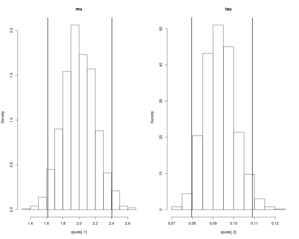
# Histogram of posterior distribution of the parameters,with 95% credibility intervals
par(mfrow=c(1,2))
hist(ajuste[,1],freq=FALSE,main="mu")
abline(v=quantile(ajuste[,1],0.025),lwd=2)
abline(v=quantile(ajuste[,1],0.975),lwd=2)
hist(ajuste[,2],freq=FALSE,main="tau")
abline(v=quantile(ajuste[,2],0.025),lwd=2)
abline(v=quantile(ajuste[,2],0.975),lwd=2)
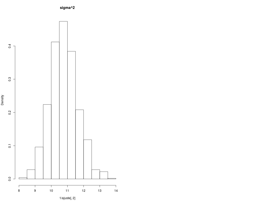
# Posterior distribution of variance sigma^2
hist(1/ajuste[,2],freq=FALSE,main="sigma^2")
# Posterior distribution of river Nile dataset
data(Nile)
postnile=posterior.normal(Nile,1000)

Results


R version 3.3.1 (2016-06-21) -- "Bug in Your Hair"
Copyright (C) 2016 The R Foundation for Statistical Computing
Platform: x86_64-pc-linux-gnu (64-bit)

R is free software and comes with ABSOLUTELY NO WARRANTY.
You are welcome to redistribute it under certain conditions.
Type 'license()' or 'licence()' for distribution details.

R is a collaborative project with many contributors.
Type 'contributors()' for more information and
'citation()' on how to cite R or R packages in publications.

Type 'demo()' for some demos, 'help()' for on-line help, or
'help.start()' for an HTML browser interface to help.
Type 'q()' to quit R.

> library(MCMC4Extremes)
Loading required package: evir
> png(filename="/home/ddbj/snapshot/RGM3/R_CC/result/MCMC4Extremes/posterior.normal.Rd_%03d_medium.png", width=480, height=480)
> ### Name: posterior.normal
> ### Title: Posterior Distribution with Normal Density
> ### Aliases: posterior.normal
> 
> ### ** Examples
> 
> # Obtaining posterior distribution of a vector of simulated points
> x=rnorm(300,2,sqrt(10))
> # Obtaning 1000 points of posterior distribution
> ajuste=posterior.normal(x,1000)
[1] 0.006666667
[1] 0.01333333
[1] 0.02
[1] 0.02666667
[1] 0.03333333
[1] 0.04
[1] 0.04666667
[1] 0.05333333
[1] 0.06
[1] 0.06666667
[1] 0.07333333
[1] 0.08
[1] 0.08666667
[1] 0.09333333
[1] 0.1
[1] 0.1066667
[1] 0.1133333
[1] 0.12
[1] 0.1266667
[1] 0.1333333
[1] 0.14
[1] 0.1466667
[1] 0.1533333
[1] 0.16
[1] 0.1666667
[1] 0.1733333
[1] 0.18
[1] 0.1866667
[1] 0.1933333
[1] 0.2
[1] 0.2066667
[1] 0.2133333
[1] 0.22
[1] 0.2266667
[1] 0.2333333
[1] 0.24
[1] 0.2466667
[1] 0.2533333
[1] 0.26
[1] 0.2666667
[1] 0.2733333
[1] 0.28
[1] 0.2866667
[1] 0.2933333
[1] 0.3
[1] 0.3066667
[1] 0.3133333
[1] 0.32
[1] 0.3266667
[1] 0.3333333
[1] 0.34
[1] 0.3466667
[1] 0.3533333
[1] 0.36
[1] 0.3666667
[1] 0.3733333
[1] 0.38
[1] 0.3866667
[1] 0.3933333
[1] 0.4
[1] 0.4066667
[1] 0.4133333
[1] 0.42
[1] 0.4266667
[1] 0.4333333
[1] 0.44
[1] 0.4466667
[1] 0.4533333
[1] 0.46
[1] 0.4666667
[1] 0.4733333
[1] 0.48
[1] 0.4866667
[1] 0.4933333
[1] 0.5
[1] 0.5066667
[1] 0.5133333
[1] 0.52
[1] 0.5266667
[1] 0.5333333
[1] 0.54
[1] 0.5466667
[1] 0.5533333
[1] 0.56
[1] 0.5666667
[1] 0.5733333
[1] 0.58
[1] 0.5866667
[1] 0.5933333
[1] 0.6
[1] 0.6066667
[1] 0.6133333
[1] 0.62
[1] 0.6266667
[1] 0.6333333
[1] 0.64
[1] 0.6466667
[1] 0.6533333
[1] 0.66
[1] 0.6666667
[1] 0.6733333
[1] 0.68
[1] 0.6866667
[1] 0.6933333
[1] 0.7
[1] 0.7066667
[1] 0.7133333
[1] 0.72
[1] 0.7266667
[1] 0.7333333
[1] 0.74
[1] 0.7466667
[1] 0.7533333
[1] 0.76
[1] 0.7666667
[1] 0.7733333
[1] 0.78
[1] 0.7866667
[1] 0.7933333
[1] 0.8
[1] 0.8066667
[1] 0.8133333
[1] 0.82
[1] 0.8266667
[1] 0.8333333
[1] 0.84
[1] 0.8466667
[1] 0.8533333
[1] 0.86
[1] 0.8666667
[1] 0.8733333
[1] 0.88
[1] 0.8866667
[1] 0.8933333
[1] 0.9
[1] 0.9066667
[1] 0.9133333
[1] 0.92
[1] 0.9266667
[1] 0.9333333
[1] 0.94
[1] 0.9466667
[1] 0.9533333
[1] 0.96
[1] 0.9666667
[1] 0.9733333
[1] 0.98
[1] 0.9866667
[1] 0.9933333
[1] 1
> # Histogram of posterior distribution of the parameters,with 95% credibility intervals
> par(mfrow=c(1,2))
> hist(ajuste[,1],freq=FALSE,main="mu")
> abline(v=quantile(ajuste[,1],0.025),lwd=2)
> abline(v=quantile(ajuste[,1],0.975),lwd=2)
> hist(ajuste[,2],freq=FALSE,main="tau")
> abline(v=quantile(ajuste[,2],0.025),lwd=2)
> abline(v=quantile(ajuste[,2],0.975),lwd=2)
> # Posterior distribution of variance sigma^2
> hist(1/ajuste[,2],freq=FALSE,main="sigma^2")
> # Posterior distribution of river Nile dataset
> data(Nile)
> postnile=posterior.normal(Nile,1000)
[1] 0.006666667
[1] 0.01333333
[1] 0.02
[1] 0.02666667
[1] 0.03333333
[1] 0.04
[1] 0.04666667
[1] 0.05333333
[1] 0.06
[1] 0.06666667
[1] 0.07333333
[1] 0.08
[1] 0.08666667
[1] 0.09333333
[1] 0.1
[1] 0.1066667
[1] 0.1133333
[1] 0.12
[1] 0.1266667
[1] 0.1333333
[1] 0.14
[1] 0.1466667
[1] 0.1533333
[1] 0.16
[1] 0.1666667
[1] 0.1733333
[1] 0.18
[1] 0.1866667
[1] 0.1933333
[1] 0.2
[1] 0.2066667
[1] 0.2133333
[1] 0.22
[1] 0.2266667
[1] 0.2333333
[1] 0.24
[1] 0.2466667
[1] 0.2533333
[1] 0.26
[1] 0.2666667
[1] 0.2733333
[1] 0.28
[1] 0.2866667
[1] 0.2933333
[1] 0.3
[1] 0.3066667
[1] 0.3133333
[1] 0.32
[1] 0.3266667
[1] 0.3333333
[1] 0.34
[1] 0.3466667
[1] 0.3533333
[1] 0.36
[1] 0.3666667
[1] 0.3733333
[1] 0.38
[1] 0.3866667
[1] 0.3933333
[1] 0.4
[1] 0.4066667
[1] 0.4133333
[1] 0.42
[1] 0.4266667
[1] 0.4333333
[1] 0.44
[1] 0.4466667
[1] 0.4533333
[1] 0.46
[1] 0.4666667
[1] 0.4733333
[1] 0.48
[1] 0.4866667
[1] 0.4933333
[1] 0.5
[1] 0.5066667
[1] 0.5133333
[1] 0.52
[1] 0.5266667
[1] 0.5333333
[1] 0.54
[1] 0.5466667
[1] 0.5533333
[1] 0.56
[1] 0.5666667
[1] 0.5733333
[1] 0.58
[1] 0.5866667
[1] 0.5933333
[1] 0.6
[1] 0.6066667
[1] 0.6133333
[1] 0.62
[1] 0.6266667
[1] 0.6333333
[1] 0.64
[1] 0.6466667
[1] 0.6533333
[1] 0.66
[1] 0.6666667
[1] 0.6733333
[1] 0.68
[1] 0.6866667
[1] 0.6933333
[1] 0.7
[1] 0.7066667
[1] 0.7133333
[1] 0.72
[1] 0.7266667
[1] 0.7333333
[1] 0.74
[1] 0.7466667
[1] 0.7533333
[1] 0.76
[1] 0.7666667
[1] 0.7733333
[1] 0.78
[1] 0.7866667
[1] 0.7933333
[1] 0.8
[1] 0.8066667
[1] 0.8133333
[1] 0.82
[1] 0.8266667
[1] 0.8333333
[1] 0.84
[1] 0.8466667
[1] 0.8533333
[1] 0.86
[1] 0.8666667
[1] 0.8733333
[1] 0.88
[1] 0.8866667
[1] 0.8933333
[1] 0.9
[1] 0.9066667
[1] 0.9133333
[1] 0.92
[1] 0.9266667
[1] 0.9333333
[1] 0.94
[1] 0.9466667
[1] 0.9533333
[1] 0.96
[1] 0.9666667
[1] 0.9733333
[1] 0.98
[1] 0.9866667
[1] 0.9933333
[1] 1
> 
> 
> 
> 
> 
> dev.off()
null device 
          1 
>