Predictive Density of GEV

Description

Predictive density resulting of posterior distribution of GEV parameters.

Usage

predictive.gev(vector, data)

Arguments

Value

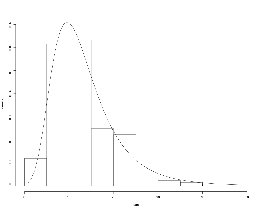
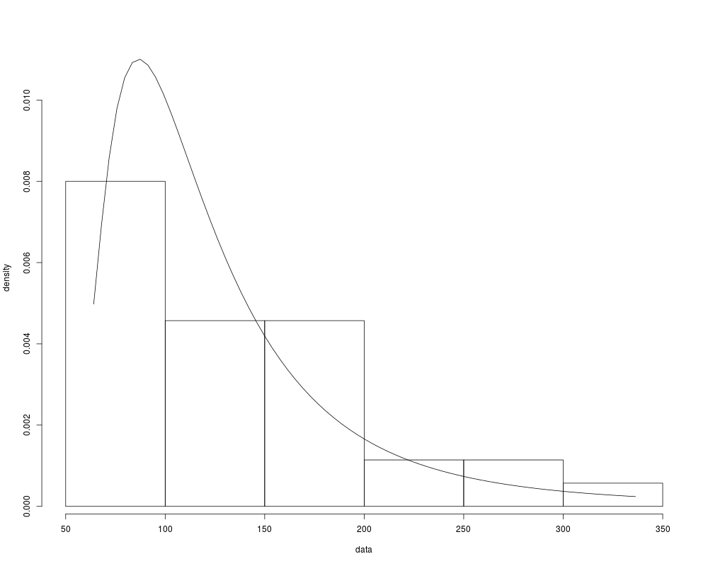
The program draws the predictive distribution of dataset fitted using the posterior distribution of the GEV parameteres.

Examples

# Fitting the predictive distribution on simulated data
x=rgev(250,xi=0.1,mu=10,sigma=5)
ajuste=posterior.gev(x,1,500)
predictive.gev(ajuste,x)
# Predictive for montly maxima of River nidd
data(nidd.annual)
out=posterior.gev(nidd.annual,1,300)
predictive.gev(out,nidd.annual)

Results

R version 3.3.1 (2016-06-21) -- "Bug in Your Hair"
Copyright (C) 2016 The R Foundation for Statistical Computing
Platform: x86_64-pc-linux-gnu (64-bit)

R is free software and comes with ABSOLUTELY NO WARRANTY.
You are welcome to redistribute it under certain conditions.
Type 'license()' or 'licence()' for distribution details.

R is a collaborative project with many contributors.
Type 'contributors()' for more information and
'citation()' on how to cite R or R packages in publications.

Type 'demo()' for some demos, 'help()' for on-line help, or
'help.start()' for an HTML browser interface to help.
Type 'q()' to quit R.

> library(MCMC4Extremes)
Loading required package: evir
> png(filename="/home/ddbj/snapshot/RGM3/R_CC/result/MCMC4Extremes/predictive.gev.Rd_%03d_medium.png", width=480, height=480)
> ### Name: predictive.gev
> ### Title: Predictive Density of GEV
> ### Aliases: predictive.gev
> 
> ### ** Examples
> 
> # Fitting the predictive distribution on simulated data
> x=rgev(250,xi=0.1,mu=10,sigma=5)
> ajuste=posterior.gev(x,1,500)
[1] 0.01333333
[1] 0.02666667
[1] 0.04
[1] 0.05333333
[1] 0.06666667
[1] 0.08
[1] 0.09333333
[1] 0.1066667
[1] 0.12
[1] 0.1333333
[1] 0.1466667
[1] 0.16
[1] 0.1733333
[1] 0.1866667
[1] 0.2
[1] 0.2133333
[1] 0.2266667
[1] 0.24
[1] 0.2533333
[1] 0.2666667
[1] 0.28
[1] 0.2933333
[1] 0.3066667
[1] 0.32
[1] 0.3333333
[1] 0.3466667
[1] 0.36
[1] 0.3733333
[1] 0.3866667
[1] 0.4
[1] 0.4133333
[1] 0.4266667
[1] 0.44
[1] 0.4533333
[1] 0.4666667
[1] 0.48
[1] 0.4933333
[1] 0.5066667
[1] 0.52
[1] 0.5333333
[1] 0.5466667
[1] 0.56
[1] 0.5733333
[1] 0.5866667
[1] 0.6
[1] 0.6133333
[1] 0.6266667
[1] 0.64
[1] 0.6533333
[1] 0.6666667
[1] 0.68
[1] 0.6933333
[1] 0.7066667
[1] 0.72
[1] 0.7333333
[1] 0.7466667
[1] 0.76
[1] 0.7733333
[1] 0.7866667
[1] 0.8
[1] 0.8133333
[1] 0.8266667
[1] 0.84
[1] 0.8533333
[1] 0.8666667
[1] 0.88
[1] 0.8933333
[1] 0.9066667
[1] 0.92
[1] 0.9333333
[1] 0.9466667
[1] 0.96
[1] 0.9733333
[1] 0.9866667
[1] 1
> predictive.gev(ajuste,x)
 [1] 0.0024650151 0.0053877956 0.0103927072 0.0178062764 0.0274170379
 [6] 0.0384801432 0.0499406781 0.0607261267 0.0699732622 0.0771365853
[11] 0.0819924350 0.0845800507 0.0851191621 0.0839305269 0.0813723419
[16] 0.0777959458 0.0735189995 0.0688122431 0.0638956740 0.0589405997
[21] 0.0540748876 0.0493895749 0.0449456778 0.0407805376 0.0369133814
[26] 0.0333499885 0.0300864798 0.0271123140 0.0244126011 0.0219698495
[31] 0.0197652567 0.0177796384 0.0159940787 0.0143903673 0.0129512776
[36] 0.0116607273 0.0105038546 0.0094670348 0.0085378562 0.0077050689
[41] 0.0069585172 0.0062890627 0.0056885038 0.0051494949 0.0046654676
[46] 0.0042305558 0.0038395259 0.0034877116 0.0031709546 0.0028855503
[51] 0.0026281990 0.0023959611 0.0021862185 0.0019966380 0.0018251404
[56] 0.0016698716 0.0015291780 0.0014015841 0.0012857722 0.0011805653
[61] 0.0010849114 0.0009978693 0.0009185968 0.0008463396 0.0007804215
[66] 0.0007202362 0.0006652396 0.0006149427 0.0005689064 0.0005267353
[71] 0.0004880738
> # Predictive for montly maxima of River nidd
> data(nidd.annual)
> out=posterior.gev(nidd.annual,1,300)
[1] 0.02222222
[1] 0.04444444
[1] 0.06666667
[1] 0.08888889
[1] 0.1111111
[1] 0.1333333
[1] 0.1555556
[1] 0.1777778
[1] 0.2
[1] 0.2222222
[1] 0.2444444
[1] 0.2666667
[1] 0.2888889
[1] 0.3111111
[1] 0.3333333
[1] 0.3555556
[1] 0.3777778
[1] 0.4
[1] 0.4222222
[1] 0.4444444
[1] 0.4666667
[1] 0.4888889
[1] 0.5111111
[1] 0.5333333
[1] 0.5555556
[1] 0.5777778
[1] 0.6
[1] 0.6222222
[1] 0.6444444
[1] 0.6666667
[1] 0.6888889
[1] 0.7111111
[1] 0.7333333
[1] 0.7555556
[1] 0.7777778
[1] 0.8
[1] 0.8222222
[1] 0.8444444
[1] 0.8666667
[1] 0.8888889
[1] 0.9111111
[1] 0.9333333
[1] 0.9555556
[1] 0.9777778
[1] 1
> predictive.gev(out,nidd.annual)
 [1] 0.0050992568 0.0069070237 0.0084878498 0.0096651258 0.0104140919
 [6] 0.0107879744 0.0108645447 0.0107199763 0.0104190917 0.0100133768
[11] 0.0095421159 0.0090344818 0.0085116730 0.0079887746 0.0074762654
[16] 0.0069811971 0.0065080957 0.0060596437 0.0056371920 0.0052411417
[21] 0.0048712285 0.0045267321 0.0042066321 0.0039097205 0.0036346848
[26] 0.0033801671 0.0031448063 0.0029272678 0.0027262625 0.0025405605
[31] 0.0023689985 0.0022104833 0.0020639937 0.0019285797 0.0018033603
[36] 0.0016875209 0.0015803101 0.0014810355 0.0013890606 0.0013038005
[41] 0.0012247183 0.0011513212 0.0010831578 0.0010198137 0.0009609096
[46] 0.0009060975 0.0008550587 0.0008075009 0.0007631562 0.0007217790
[51] 0.0006831439 0.0006470441 0.0006132899 0.0005817069 0.0005521350
[56] 0.0005244271 0.0004984479 0.0004740729 0.0004511875 0.0004296862
[61] 0.0004094717 0.0003904543 0.0003725515 0.0003556867 0.0003397897
[66] 0.0003247951 0.0003106429 0.0002972772 0.0002846465 0.0002727030
[71] 0.0002614025
> 
> 
> 
> 
> 
> dev.off()
null device 
          1 
>