Markov chain Monte Carlo Sampler for Multivariate Generalised Linear Mixed
Models with special emphasis on correlated random effects arising from pedigrees
and phylogenies (Hadfield 2010). Please read the course notes: vignette("CourseNotes",
"MCMCglmm") or the overview vignette("Overview", "MCMCglmm")
formula for the fixed effects, multiple responses
are passed as a matrix using cbind
random
formula for the random effects. Multiple random terms can be passed using the + operator, and in the most general case each random term has the form variance.function(formula):linking.function(random.terms). Currently, the only variance.functions available are idv, idh, us, cor[] and ante[]. idv fits a constant variance across all components in formula. Both idh and us fit different variances across each component in formula, but us will also fit the covariances. corg fixes the variances along the diagonal to one and corgh fixes the variances along the diagonal to those specified in the prior. cors allows correlation submatrices.
ante[] fits ante-dependence structures of different order (e.g ante1, ante2), and the number can be prefixed by a c to hold all regression coefficients of the same order equal. The number can also be suffixed by a v to hold all innovation variances equal (e.g antec2v has 3 parameters). The formula can contain both factors and numeric terms (i.e. random regression) although it should be noted that the intercept term is suppressed. The (co)variances are the (co)variances of the random.terms effects. Currently, the only linking.functions available are mm and str. mm fits a multimembership model where multiple random terms are separated by the + operator. str allows covariances to exist between multiple random terms that are also separated by the + operator. In both cases the levels of all multiple random terms have to be the same. For simpler models the variance.function(formula) and linking.function(random.terms) can be omitted and the model syntax has the simpler form ~random1+random2+.... There are two reserved variables: units which index rows of the response variable and trait which index columns of the response variable
rcov
formula for residual covariance structure. This has to be set up so that each data point is associated with a unique residual. For example a multi-response model might have the R-structure defined by ~us(trait):units
family
optional character vector of trait distributions. Currently,
"gaussian", "poisson", "categorical",
"multinomial", "ordinal", "threshold", "exponential", "geometric", "cengaussian",
"cenpoisson", "cenexponential", "zipoisson", "zapoisson", "ztpoisson", "hupoisson", "zibinomial" and "threshold" are
supported, where the prefix "cen" means censored, the prefix "zi" means zero inflated, the prefix "za" means zero altered, the prefix "zt" means zero truncated and the prefix "hu" means hurdle. If NULL, data needs to contain a
family column.
mev
optional vector of measurement error variances for each data point
for random effect meta-analysis.
data
data.frame
start
optional list having 4 possible elements:
R (R-structure) G (G-structure) and liab (latent variables or liabilities) should contain the starting values where G itself is also a list with as many elements as random effect components. The fourth element QUASI should be logical: if TRUE starting latent variables are obtained heuristically, if FALSE then they are sampled from a Z-distribution
prior
optional list of prior specifications having 3 possible elements:
R (R-structure) G (G-structure) and B (fixed effects). B is a list containing the expected value (mu) and a
(co)variance matrix (V) representing the strength of belief: the defaults are B$mu=0 and B$V=I*1e+10, where where I is an identity matrix of appropriate dimension. The priors for the variance structures (R and G) are lists with the expected (co)variances (V) and degree of belief parameter (nu) for the inverse-Wishart, and also the mean vector (alpha.mu) and covariance matrix (alpha.V) for the redundant working parameters. The defaults are nu=0, V=1, alpha.mu=0, and alpha.V=0. When alpha.V is non-zero, parameter expanded algorithms are used.
tune
optional (co)variance matrix defining the proposal distribution
for the latent variables. If NULL an adaptive algorithm is used which ceases to
adapt once the burn-in phase has finished.
pedigree
ordered pedigree with 3 columns id, dam and sire or a
phylo object. This argument is retained for back compatibility - see ginverse argument for a more general formulation.
nodes
pedigree/phylogeny nodes to be estimated. The default,
"ALL" estimates effects for all individuals in a pedigree or nodes in a
phylogeny (including ancestral nodes). For phylogenies "TIPS" estimates
effects for the tips only, and for pedigrees a vector of ids can be passed to
nodes specifying the subset of individuals for which animal effects are
estimated. Note that all analyses are equivalent if omitted nodes have missing
data but by absorbing these nodes the chain max mix better. However, the
algorithm may be less numerically stable and may iterate slower, especially for
large phylogenies.
scale
logical: should the phylogeny (needs to be ultrametric) be scaled
to unit length (distance from root to tip)?
nitt
number of MCMC iterations
thin
thinning interval
burnin
burnin
pr
logical: should the posterior distribution of random effects be
saved?
pl
logical: should the posterior distribution of latent variables be
saved?
verbose
logical: if TRUE MH diagnostics are printed to screen
DIC
logical: if TRUE deviance and deviance information criterion are calculated
singular.ok
logical: if FALSE linear dependencies in the fixed effects are removed. if TRUE they are left in an estimated, although all information comes form the prior
saveX
logical: save fixed effect design matrix
saveZ
logical: save random effect design matrix
saveXL
logical: save structural parameter design matrix
slice
logical: should slice sampling be used? Only applicable for binary traits with independent residuals
ginverse
a list of sparse inverse matrices (solve(A)) that are proportional to the covariance structure of the random effects. The names of the matrices should correspond to columns in data that are associated with the random term. All levels of the random term should appear as rownames for the matrices.
Value
Sol
Posterior Distribution of MME solutions, including fixed effects
VCV
Posterior Distribution of (co)variance matrices
CP
Posterior Distribution of cut-points from an ordinal model
Liab
Posterior Distribution of latent variables
Fixed
list: fixed formula and number of fixed effects
Random
list: random formula, dimensions of each covariance matrix, number of levels per covariance matrix, and term in random formula to which each covariance belongs
Residual
list: residual formula, dimensions of each covariance matrix, number of levels per covariance matrix, and term in residual formula to which each covariance belongs
Deviance
deviance -2*log(p(y|...))
DIC
deviance information criterion
X
sparse fixed effect design matrix
Z
sparse random effect design matrix
XL
sparse structural parameter design matrix
error.term
residual term for each datum
family
distribution of each datum
Tune
(co)variance matrix of the proposal distribution for the latent variables
General analyses: Hadfield, J.D. (2010) Journal of Statistical Software 33 2 1-22
Phylogenetic analyses: Hadfield, J.D. & Nakagawa, S. (2010) Journal of Evolutionary Biology 23 494-508
Background Sorensen, D. & Gianola, D. (2002) Springer
See Also
mcmc
Examples
# Example 1: univariate Gaussian model with standard random effect

data(PlodiaPO)
model1<-MCMCglmm(PO~1, random=~FSfamily, data=PlodiaPO, verbose=FALSE)
summary(model1)

# Example 2: univariate Gaussian model with phylogenetically correlated
# random effect

data(bird.families)

phylo.effect<-rbv(bird.families, 1, nodes="TIPS")
phenotype<-phylo.effect+rnorm(dim(phylo.effect)[1], 0, 1)

# simulate phylogenetic and residual effects with unit variance

test.data<-data.frame(phenotype=phenotype, taxon=row.names(phenotype))

Ainv<-inverseA(bird.families)$Ainv

# inverse matrix of shared phyloegnetic history

prior<-list(R=list(V=1, nu=0.002), G=list(G1=list(V=1, nu=0.002)))

model2<-MCMCglmm(phenotype~1, random=~taxon, ginverse=list(taxon=Ainv),
data=test.data, prior=prior, verbose=FALSE)

plot(model2$VCV)
Results
R version 3.3.1 (2016-06-21) -- "Bug in Your Hair"
Copyright (C) 2016 The R Foundation for Statistical Computing
Platform: x86_64-pc-linux-gnu (64-bit)
R is free software and comes with ABSOLUTELY NO WARRANTY.
You are welcome to redistribute it under certain conditions.
Type 'license()' or 'licence()' for distribution details.
R is a collaborative project with many contributors.
Type 'contributors()' for more information and
'citation()' on how to cite R or R packages in publications.
Type 'demo()' for some demos, 'help()' for on-line help, or
'help.start()' for an HTML browser interface to help.
Type 'q()' to quit R.
> library(MCMCglmm)
Loading required package: Matrix
Loading required package: coda
Loading required package: ape
> png(filename="/home/ddbj/snapshot/RGM3/R_CC/result/MCMCglmm/MCMCglmm.Rd_%03d_medium.png", width=480, height=480)
> ### Name: MCMCglmm
> ### Title: Multivariate Generalised Linear Mixed Models
> ### Aliases: MCMCglmm
> ### Keywords: models
>
> ### ** Examples
>
>
> # Example 1: univariate Gaussian model with standard random effect
>
> data(PlodiaPO)
> model1<-MCMCglmm(PO~1, random=~FSfamily, data=PlodiaPO, verbose=FALSE)
> summary(model1)
Iterations = 3001:12991
Thinning interval = 10
Sample size = 1000
DIC: -239.9547
G-structure: ~FSfamily
post.mean l-95% CI u-95% CI eff.samp
FSfamily 0.01004 0.004943 0.01595 1000
R-structure: ~units
post.mean l-95% CI u-95% CI eff.samp
units 0.03397 0.02968 0.03838 1127
Location effects: PO ~ 1
post.mean l-95% CI u-95% CI eff.samp pMCMC
(Intercept) 1.164 1.134 1.195 1000 <0.001 ***
---
Signif. codes: 0 '***' 0.001 '**' 0.01 '*' 0.05 '.' 0.1 ' ' 1
>
> # Example 2: univariate Gaussian model with phylogenetically correlated
> # random effect
>
> data(bird.families)
>
> phylo.effect<-rbv(bird.families, 1, nodes="TIPS")
> phenotype<-phylo.effect+rnorm(dim(phylo.effect)[1], 0, 1)
>
> # simulate phylogenetic and residual effects with unit variance
>
> test.data<-data.frame(phenotype=phenotype, taxon=row.names(phenotype))
>
> Ainv<-inverseA(bird.families)$Ainv
>
> # inverse matrix of shared phyloegnetic history
>
> prior<-list(R=list(V=1, nu=0.002), G=list(G1=list(V=1, nu=0.002)))
>
> model2<-MCMCglmm(phenotype~1, random=~taxon, ginverse=list(taxon=Ainv),
+ data=test.data, prior=prior, verbose=FALSE)
>
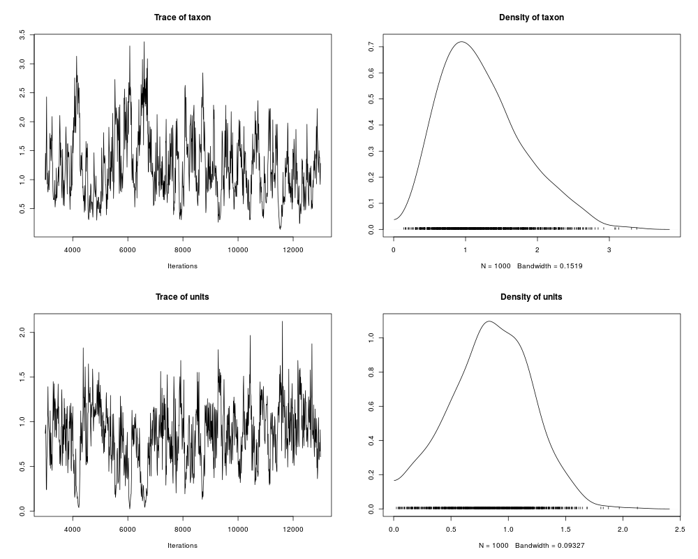
> plot(model2$VCV)
>
>
>
>
>
>
> dev.off()
null device
1
>
 .
.