R Graphical Manual

Browse All

Last data update: 2014.03.03

R: Markov Chain Monte Carlo for Ordered Probit Changepoint...

MCMCoprobitChange

R Documentation

Markov Chain Monte Carlo for Ordered Probit Changepoint Regression Model

Description

This function generates a sample from the posterior distribution of an ordered probit regression model with multiple parameter breaks. The function uses the Markov chain Monte Carlo method of Chib (1998). The user supplies data and priors, and a sample from the posterior distribution is returned as an mcmc object, which can be subsequently analyzed with functions provided in the coda package.

Usage

MCMCoprobitChange(formula, data=parent.frame(),  m = 1,
        burnin = 1000, mcmc = 1000, thin = 1, tune = NA, verbose = 0,
        seed = NA, beta.start = NA, gamma.start=NA, P.start = NA,
        b0 = NULL, B0 = NULL, a = NULL, b = NULL,
        marginal.likelihood = c("none", "Chib95"), gamma.fixed=0, ...)

Arguments

`formula`	Model formula.
`data`	Data frame.
`m`	The number of changepoints.
`burnin`	The number of burn-in iterations for the sampler.
`mcmc`	The number of MCMC iterations after burnin.
`thin`	The thinning interval used in the simulation. The number of MCMC iterations must be divisible by this value.
`tune`	The tuning parameter for the Metropolis-Hastings step. Default of NA corresponds to a choice of 0.05 divided by the number of categories in the response variable.
`verbose`	A switch which determines whether or not the progress of the sampler is printed to the screen. If `verbose` is greater than 0 the iteration number, the beta vector, and the error variance are printed to the screen every `verbose`th iteration.
`seed`	The seed for the random number generator. If NA, the Mersenne Twister generator is used with default seed 12345; if an integer is passed it is used to seed the Mersenne twister. The user can also pass a list of length two to use the L'Ecuyer random number generator, which is suitable for parallel computation. The first element of the list is the L'Ecuyer seed, which is a vector of length six or NA (if NA a default seed of `rep(12345,6)` is used). The second element of list is a positive substream number. See the MCMCpack specification for more details.
`beta.start`	The starting values for the beta vector. This can either be a scalar or a column vector with dimension equal to the number of betas. The default value of of NA will use the MLE estimate of beta as the starting value. If this is a scalar, that value will serve as the starting value mean for all of the betas.
`gamma.start`	The starting values for the gamma vector. This can either be a scalar or a column vector with dimension equal to the number of gammas. The default value of of NA will use the MLE estimate of gamma as the starting value. If this is a scalar, that value will serve as the starting value mean for all of the gammas.
`P.start`	The starting values for the transition matrix. A user should provide a square matrix with dimension equal to the number of states. By default, draws from the `Beta(0.9, 0.1)` are used to construct a proper transition matrix for each raw except the last raw.
`b0`	The prior mean of beta. This can either be a scalar or a column vector with dimension equal to the number of betas. If this takes a scalar value, then that value will serve as the prior mean for all of the betas.
`B0`	The prior precision of beta. This can either be a scalar or a square matrix with dimensions equal to the number of betas. If this takes a scalar value, then that value times an identity matrix serves as the prior precision of beta. Default value of 0 is equivalent to an improper uniform prior for beta.
`a`	a is the shape1 beta prior for transition probabilities. By default, the expected duration is computed and corresponding a and b values are assigned. The expected duration is the sample period divided by the number of states.
`b`	b is the shape2 beta prior for transition probabilities. By default, the expected duration is computed and corresponding a and b values are assigned. The expected duration is the sample period divided by the number of states.
`marginal.likelihood`	How should the marginal likelihood be calculated? Options are: `none` in which case the marginal likelihood will not be calculated, and `Chib95` in which case the method of Chib (1995) is used.
`gamma.fixed`	1 if users want to constrain gamma values to be constant. By default, gamma values are allowed to vary across regimes.
`...`	further arguments to be passed

Details

MCMCoprobitChange simulates from the posterior distribution of an ordinal probit regression model with multiple parameter breaks. The simulation of latent states is based on the linear approximation method discussed in Park (2011).

The model takes the following form:

Pr(y_t = 1) = Phi(gamma_(c, m) - x_i'beta_m) - Phi(gamma_(c-1, m) - x_i'beta)

Where M is the number of states, and gamma_(c, m) and beta_m are paramters when a state is m at t.

We assume Gaussian distribution for prior of beta:

beta_m ~ N(b0,B0^(-1)), m = 1,...,M.

And:

p_mm ~ Beta(a, b), m = 1,...,M.

Where M is the number of states.

Note that when the fitted changepoint model has very few observations in any of states, the marginal likelihood outcome can be “nan," which indicates that too many breaks are assumed given the model and data.

Value

An mcmc object that contains the posterior sample. This object can be summarized by functions provided by the coda package. The object contains an attribute prob.state storage matrix that contains the probability of state_i for each period, the log-likelihood of the model (loglike), and the log-marginal likelihood of the model (logmarglike).

References

Jong Hee Park. 2011. “Changepoint Analysis of Binary and Ordinal Probit Models: An Application to Bank Rate Policy Under the Interwar Gold Standard." Political Analysis. 19: 188-204.

Andrew D. Martin, Kevin M. Quinn, and Jong Hee Park. 2011. “MCMCpack: Markov Chain Monte Carlo in R.”, Journal of Statistical Software. 42(9): 1-21. http://www.jstatsoft.org/v42/i09/.

Siddhartha Chib. 1998. “Estimation and comparison of multiple change-point models.” Journal of Econometrics. 86: 221-241.

Examples

set.seed(1909)
N <- 200
x1 <- rnorm(N, 1, .5);

## set a true break at 100
z1 <- 1 + x1[1:100] + rnorm(100);
z2 <- 1 -0.2*x1[101:200] + rnorm(100);
z <- c(z1,  z2);
y <- z

## generate y
y[z < 1] <- 1;
y[z >= 1 & z < 2] <- 2;
y[z >= 2] <- 3;

## inputs
formula <- y ~ x1 

## fit multiple models with a varying number of breaks
out1 <- MCMCoprobitChange(formula, m=1, 
      	mcmc=100, burnin=100, thin=1, tune=c(.5, .5), verbose=100, 
     	b0=0, B0=10, marginal.likelihood = "Chib95")
out2 <- MCMCoprobitChange(formula, m=2, 
      	mcmc=100, burnin=100, thin=1, tune=c(.5, .5, .5), verbose=100, 
     	b0=0, B0=10, marginal.likelihood = "Chib95")

## Do model comparison
## NOTE: the chain should be run longer than this example!
BayesFactor(out1, out2)

## draw plots using the "right" model
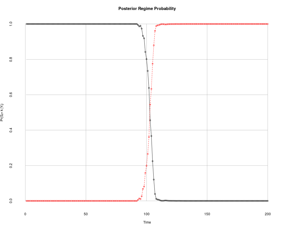
plotState(out1)
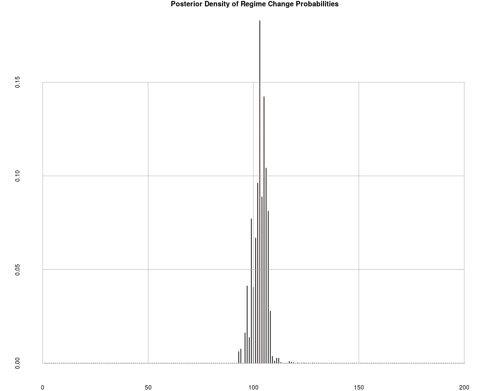
plotChangepoint(out1)

Results


R version 3.3.1 (2016-06-21) -- "Bug in Your Hair"
Copyright (C) 2016 The R Foundation for Statistical Computing
Platform: x86_64-pc-linux-gnu (64-bit)

R is free software and comes with ABSOLUTELY NO WARRANTY.
You are welcome to redistribute it under certain conditions.
Type 'license()' or 'licence()' for distribution details.

R is a collaborative project with many contributors.
Type 'contributors()' for more information and
'citation()' on how to cite R or R packages in publications.

Type 'demo()' for some demos, 'help()' for on-line help, or
'help.start()' for an HTML browser interface to help.
Type 'q()' to quit R.

> library(MCMCpack)
Loading required package: coda
Loading required package: MASS
##
## Markov Chain Monte Carlo Package (MCMCpack)
## Copyright (C) 2003-2016 Andrew D. Martin, Kevin M. Quinn, and Jong Hee Park
##
## Support provided by the U.S. National Science Foundation
## (Grants SES-0350646 and SES-0350613)
##
> png(filename="/home/ddbj/snapshot/RGM3/R_CC/result/MCMCpack/MCMCoprobitChange.Rd_%03d_medium.png", width=480, height=480)
> ### Name: MCMCoprobitChange
> ### Title: Markov Chain Monte Carlo for Ordered Probit Changepoint
> ###   Regression Model
> ### Aliases: MCMCoprobitChange
> ### Keywords: models
> 
> ### ** Examples
> 
> set.seed(1909)
> N <- 200
> x1 <- rnorm(N, 1, .5);
> 
> ## set a true break at 100
> z1 <- 1 + x1[1:100] + rnorm(100);
> z2 <- 1 -0.2*x1[101:200] + rnorm(100);
> z <- c(z1,  z2);
> y <- z
> 
> ## generate y
> y[z < 1] <- 1;
> y[z >= 1 & z < 2] <- 2;
> y[z >= 2] <- 3;
> 
> ## inputs
> formula <- y ~ x1 
> 
> ## fit multiple models with a varying number of breaks
> out1 <- MCMCoprobitChange(formula, m=1, 
+       	mcmc=100, burnin=100, thin=1, tune=c(.5, .5), verbose=100, 
+      	b0=0, B0=10, marginal.likelihood = "Chib95")


MCMCoprobitChange iteration 101 of 200 


 Acceptance rate for state 1 is    0.53000 


 Acceptance rate for state 2 is    0.20000 

 The number of observations in state 1 is      00097
 The number of observations in state 2 is      00103
 beta 0 =    0.09304   0.52479
 beta 1 =   -0.27336   0.16873
 gamma 0 =    0.74271
 gamma 1 =    0.99581
logmarglike = -220.60851
loglike = -192.32574
log_prior =   -4.61781
log_beta =    4.33846
log_P =    3.63139
log_gamma =   15.69512
> out2 <- MCMCoprobitChange(formula, m=2, 
+       	mcmc=100, burnin=100, thin=1, tune=c(.5, .5, .5), verbose=100, 
+      	b0=0, B0=10, marginal.likelihood = "Chib95")


MCMCoprobitChange iteration 101 of 200 


 Acceptance rate for state 1 is    0.61000 


 Acceptance rate for state 2 is    0.81000 


 Acceptance rate for state 3 is    0.21000 

 The number of observations in state 1 is      00001
 The number of observations in state 2 is      00001
 The number of observations in state 3 is      00198
 beta 0 =    0.09056   0.25382
 beta 1 =   -0.54118  -0.45300
 beta 2 =   -0.33464   0.54185
 gamma 0 =    0.92141
 gamma 1 =    1.23897
 gamma 2 =    0.70838
logmarglike = -241.98699
loglike = -212.84326
log_prior =   -8.97530
log_beta =    3.75571
log_P =    2.18454
log_gamma =   14.22818
> 
> ## Do model comparison
> ## NOTE: the chain should be run longer than this example!
> BayesFactor(out1, out2)
The matrix of Bayes Factors is:
         out1     out2
out1 1.00e+00 1.93e+09
out2 5.19e-10 1.00e+00

The matrix of the natural log Bayes Factors is:
      out1 out2
out1   0.0 21.4
out2 -21.4  0.0

 out1 :
   call = 
MCMCoprobitChange(formula = formula, m = 1, burnin = 100, mcmc = 100, 
    thin = 1, tune = c(0.5, 0.5), verbose = 100, b0 = 0, B0 = 10, 
    marginal.likelihood = "Chib95")

   log marginal likelihood =  -220.6085 


 out2 :
   call = 
MCMCoprobitChange(formula = formula, m = 2, burnin = 100, mcmc = 100, 
    thin = 1, tune = c(0.5, 0.5, 0.5), verbose = 100, b0 = 0, 
    B0 = 10, marginal.likelihood = "Chib95")

   log marginal likelihood =  -241.987 

> 
> ## draw plots using the "right" model
> plotState(out1)
> plotChangepoint(out1)
> 
> 
> 
> 
> 
> dev.off()
null device 
          1 
>