R Graphical Manual

Browse All

Last data update: 2014.03.03

R: Confidence intervals for multiple contrasts of Shannon...

Shannonci

R Documentation

Confidence intervals for multiple contrasts of Shannon indices

Description

Calculates simultaneous and local confidence intervals for differences of Shannon indices under the assumption of multinomial count data.

Usage

Shannonci(X, f, cmat = NULL, type = "Dunnett", alternative = "two.sided",
 conf.level = 0.95, dist = "MVN", ...)

Arguments

`X`	a data.frame of dimensions n times p with integer entries, where n is the number of samples and p is the number of species
`f`	a factor variable of length n, grouping the observations in `X`
`cmat`	an contrast matrix; the number of columns should match the number of levels in `f`
`type`	a single character string, currently one of "Dunnett","Tukey","Sequen"
`alternative`	a single character string, one of "two.sided","less" (upper bounds),"greater" (lower bounds)
`conf.level`	the confidence level of the simultaneous (or local) confidence intervals
`dist`	a single character string, defining the type of quantiles to be used for interval calculation; "MVN" invokes simultaneous intervals, "N" invokes unadjusted confidence intervals with coverage probability conf.level for each of them
`...`	further arguments to be passed; currently only `base` is used, a single integer value, specifying which group to be taken as the control in case that `type="Dunnett"`, ignored otherwise

Details

This function implements confidence intervals described by Fritsch and Hsu (1999) for the difference of Shannon indices between several groups. Deviating from Fritsch and Hsu, quantiles of the multivariate normal distribution based on a plug-in-estamator for the correlation matrix.

Note, that this approach, by assuming multinomial distribution for the vectors of counts, ignores the variability of the individual samples. If such extra-multinomial variatio is present in the data, the intervals will be too narrow, coverage probability will be substantially lower than specified in 'conf.level'. Consider approaches based on bootstrap instead (e.g., package simboot).

Value

A list containing the elements:

`conf.int`	a matrix, containing the lower and upper confidence limits in the columns
`quantile`	a single numeric value, the quantile used for interval calculation
`estimate`	a matrix,containing the point estimates of the contrasts in its column
`cmat`	the contrast matrix used
`methodname`	a character string, for printing
`sample.estimate`	A list of sample estimates as returned by estShannonf

and some of the input arguments

Author(s)

Frank Schaarschmidt

References

Fritsch, KS, and Hsu, JC (1999): Multiple Comparison of Entropies with Application to Dinosaur Biodiversity. Biometrics 55, 1300-1305. Scherer, R, Schaarschmidt, F, Prescher, S, and Priesnitz, KU (2013): Simultaneous confidence intervals for comparing biodiversity indices estimated from overdispersed count data. Biometrical Journal 55,246-263.

Examples



data(HCD)

HCDcounts<-HCD[,-1]
HCDf<-HCD[,1]

# Comparison to the confidence bounds shown in
# Fritsch and Hsu (1999), Table 5, "Standard normal".

cmat<-rbind(
"HM-HU"=c(0,1,-1),
"HL-HM"=c(1,-1,0),
"HL-HU"=c(1,0,-1)
)

Shannonci(X=HCDcounts, f=HCDf, cmat=cmat,
 alternative = "two.sided", conf.level = 0.9, dist = "N")

# Note, that the calculated confidence intervals
# differ from those published by Fritsch and Hsu (1999),
# whenever Lower is involved.



# Comparison to the lower cretaceous,
# unadjusted confidence intervals:

Shannonci(X=HCDcounts, f=HCDf, type = "Dunnett",
 alternative = "greater", conf.level = 0.9, dist = "N")

# Stepwise comparison between the strata,
# unadjusted confidence intervals:

ShannonS<-Shannonci(X=HCDcounts, f=HCDf, type = "Sequen",
 alternative = "greater", conf.level = 0.9, dist = "N")


ShannonS

summary(ShannonS)

plot(ShannonS)


# A trend test based on multiple contrasts:

cmatTREND<-rbind(
"U-LM"=c(-0.5,-0.5,1),
"MU-L"=c(-1,0.5,0.5),
"U-L"=c(-1,0,1)
)

TrendCI<-Shannonci(X=HCDcounts, f=HCDf, cmat=cmatTREND,
 alternative = "greater", conf.level = 0.95, dist = "MVN")
TrendCI

plot(TrendCI)

Results


R version 3.3.1 (2016-06-21) -- "Bug in Your Hair"
Copyright (C) 2016 The R Foundation for Statistical Computing
Platform: x86_64-pc-linux-gnu (64-bit)

R is free software and comes with ABSOLUTELY NO WARRANTY.
You are welcome to redistribute it under certain conditions.
Type 'license()' or 'licence()' for distribution details.

R is a collaborative project with many contributors.
Type 'contributors()' for more information and
'citation()' on how to cite R or R packages in publications.

Type 'demo()' for some demos, 'help()' for on-line help, or
'help.start()' for an HTML browser interface to help.
Type 'q()' to quit R.

> library(MCPAN)
> png(filename="/home/ddbj/snapshot/RGM3/R_CC/result/MCPAN/Shannonci.Rd_%03d_medium.png", width=480, height=480)
> ### Name: Shannonci
> ### Title: Confidence intervals for multiple contrasts of Shannon indices
> ### Aliases: Shannonci
> ### Keywords: htest
> 
> ### ** Examples
> 
> 
> 
> data(HCD)
> 
> HCDcounts<-HCD[,-1]
> HCDf<-HCD[,1]
> 
> # Comparison to the confidence bounds shown in
> # Fritsch and Hsu (1999), Table 5, "Standard normal".
> 
> cmat<-rbind(
+ "HM-HU"=c(0,1,-1),
+ "HL-HM"=c(1,-1,0),
+ "HL-HU"=c(1,0,-1)
+ )
> 
> Shannonci(X=HCDcounts, f=HCDf, cmat=cmat,
+  alternative = "two.sided", conf.level = 0.9, dist = "N")
Local 90 percent-confidence intervals 
 for differences of Shannon indices 
      estimate   lower  upper
HM-HU   0.0934 -0.1061 0.2928
HL-HM   0.0160 -0.2627 0.2947
HL-HU   0.1094 -0.1847 0.4035
> 
> # Note, that the calculated confidence intervals
> # differ from those published by Fritsch and Hsu (1999),
> # whenever Lower is involved.
> 
> 
> 
> # Comparison to the lower cretaceous,
> # unadjusted confidence intervals:
> 
> Shannonci(X=HCDcounts, f=HCDf, type = "Dunnett",
+  alternative = "greater", conf.level = 0.9, dist = "N")
Local 90 percent-confidence intervals 
 for differences of Shannon indices 
               estimate   lower upper
Middle - Lower  -0.0160 -0.2332   Inf
Upper - Lower   -0.1094 -0.3385   Inf
> 
> # Stepwise comparison between the strata,
> # unadjusted confidence intervals:
> 
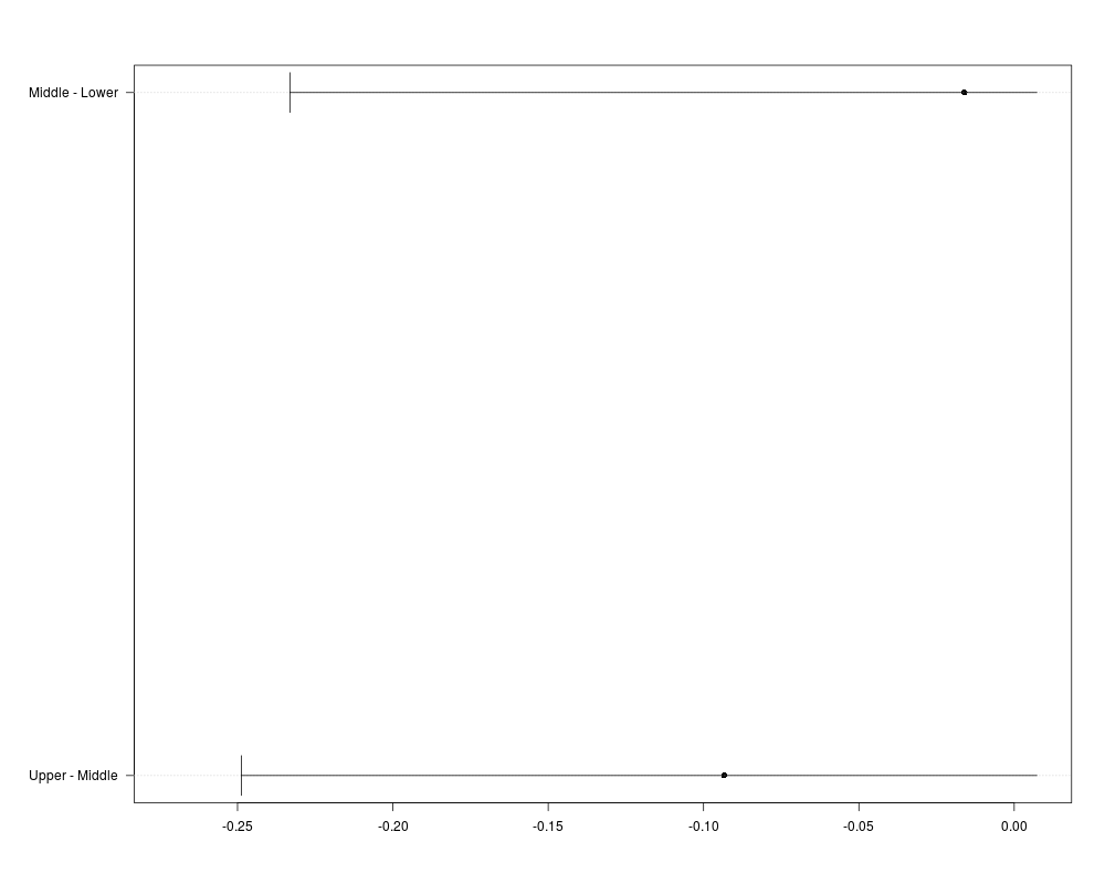
> ShannonS<-Shannonci(X=HCDcounts, f=HCDf, type = "Sequen",
+  alternative = "greater", conf.level = 0.9, dist = "N")
> 
> 
> ShannonS
Local 90 percent-confidence intervals 
 for differences of Shannon indices 
               estimate   lower upper
Middle - Lower  -0.0160 -0.2332   Inf
Upper - Middle  -0.0934 -0.2488   Inf
> 
> summary(ShannonS)

 Data: 
       Cr Ha Hy Pa Ty Or Sa Dr
Lower  19  7  1  0  2  0  3  0
Middle 53 51  2  0  3  8  6  0
Upper  50 29  3  0  3  4  1  0

 Summary statistics: 
                                        Lower   Middle  Upper
Total number of individuals            32.000 123.0000 90.000
Shannon index, bias corrected estimate  1.255   1.2389  1.145
Shannon index, raw estimate             1.145   1.2104  1.107
Variance estimate                       0.023   0.0057  0.009

 Contrast matrix: 

	 Multiple Comparisons of Means: Sequen Contrasts

               Lower Middle Upper
Middle - Lower    -1      1     0
Upper - Middle     0     -1     1

Local 90 percent-confidence intervals 
 for differences of Shannon indices 
               estimate   lower upper
Middle - Lower  -0.0160 -0.2332   Inf
Upper - Middle  -0.0934 -0.2488   Inf
> 
> plot(ShannonS)
> 
> 
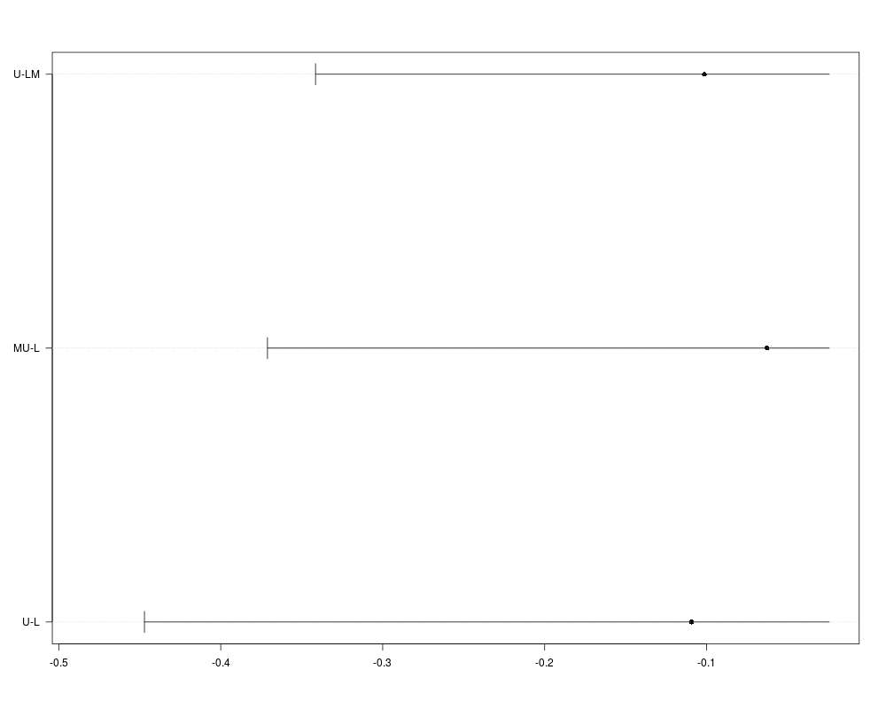
> # A trend test based on multiple contrasts:
> 
> cmatTREND<-rbind(
+ "U-LM"=c(-0.5,-0.5,1),
+ "MU-L"=c(-1,0.5,0.5),
+ "U-L"=c(-1,0,1)
+ )
> 
> TrendCI<-Shannonci(X=HCDcounts, f=HCDf, cmat=cmatTREND,
+  alternative = "greater", conf.level = 0.95, dist = "MVN")
> TrendCI
Simultaneous 95 percent-confidence intervals 
 for differences of Shannon indices 
     estimate   lower upper
U-LM  -0.1014 -0.3417   Inf
MU-L  -0.0627 -0.3714   Inf
U-L   -0.1094 -0.4474   Inf
> 
> plot(TrendCI)
> 
> 
> 
>   
> 
> 
> 
> 
> dev.off()
null device 
          1 
>