R Graphical Manual

Browse All

Last data update: 2014.03.03

R: Simultaneous confidence intervals for odds ratios

binomORci

R Documentation

Simultaneous confidence intervals for odds ratios

Description

Approximate simultaneous confidence intervals for (weighted geometric means of) odds ratios are constructed. Estimates are derived from fitting a glm on the logit-link, approximate intervals are constructed on the logit-link, and transformed to original scale.

Usage

binomORci(x, ...)

## Default S3 method:
binomORci(x, n, names = NULL,
 type = "Dunnett", method="GLM", cmat = NULL,
 alternative = "two.sided", conf.level = 0.95,
 dist="MVN", ...)

## S3 method for class 'formula'
binomORci(formula, data,
 type = "Dunnett", method="GLM", cmat = NULL,
 alternative = "two.sided", conf.level = 0.95,
 dist="MVN", ...)

## S3 method for class 'table'
binomORci(x,
 type = "Dunnett",method="GLM", cmat = NULL,
 alternative = "two.sided", conf.level = 0.95,
 dist="MVN", ...)

## S3 method for class 'matrix'
binomORci(x,
 type = "Dunnett", method="GLM", cmat = NULL,
 alternative = "two.sided", conf.level = 0.95,
 dist="MVN", ...)

Arguments

`x`	a numeric vector, giving the number of successes in I independent samples, or an object of class `"table"`, representing the 2xk-table, or an object of class `"matrix"`, representing the 2xk-table
`n`	numeric vector, giving the number of trials (i.e. the sample size) in each of the I groups (only required if `x` is a numeric vector, ignored otherwise)
`names`	an optional character string, giving the names of the groups/ sample in `x`, `n`; if not specified the possible names of x are taken as group names (ignored if `x` is a table or matrix)
`formula`	a two-sided formula of the style 'response ~ treatment', where 'response' should be a categorical variable with two levels, while treatment should be a factor specifying the treatment levels
`data`	a data.frame, containing the variables specified in formula
`type`	a character string, giving the name of a contrast method, as defined in `contrMat(multcomp)`; ignored if `cmat` is sepcified
`method`	a single character string, specifying the method for confidence interval computation; Options are `"GLM"` and `"Woolf"`. `"GLM"` takes the maximum likelihood estimates and the their standard errors; this yields a conservative confidence intervals with uninformative limits if x=0 and x=n occures. `"Woolf"` adds 0.5 to the cell counts, resulting in less conservative bounds. These can be liberal when extreme proportions are compared.
`cmat`	a optional contrast matrix
`alternative`	a single character string, one of "two.sided", "less", "greater"
`conf.level`	a single numeric value, simultaneous confidence level
`dist`	a character string, `"MVN"` invokes multiplicity adjustment via the multivariate normal distribution, `"N"` invokes use of quantiles of the univariate normal distribution
`...`	arguments to be passed to binomest, currently only `success` labelling the event which should be considered as success

Details

This function calls glm and fits a one-way-model with family binomial on the logit-link. Then, the point estimates and variances estimates from the fit are taken to construct simultaneous confidence intervals for differences (of weighted arithmetic means) of log-odds. Applying the exponential function to these intervals on the logit scale yields intervals for ratios (of weighted geometric) of odds. For simple groupwise comparisons, one yields intervals for oddsratios. For the case of Dunnett-type contrasts, the calculated simultaneous confidence intervals are those described in Holford et al. (1989).

Specifying method="GLM" takes maximum likelihood estimates for the log-odds and their standard errors evaluated at the estimate.

Specifying method="Woolf" takes adds 0.5 to each cell count and computes point estimates and standard errors for these continuity corrected values. For the two-sample comparison this method is refered to as "adjusted Woolf" (Lawson, 2005). In this implementation, the lower bounds yielded by this method are additionally expanded to 0, if all values in the denominator are x=n or all values in the numerator are x=0, and the upper bounds are expanded to Inf, if all values in the denominator are x=0 or all values in the numerator are x=n.

Note, that for the case of general contrasts, the methods are not described explicitly so far.

Value

A object of class "binomORci", a list containing:

`conf.int`	a matrix with 2 columns: lower and upper confidence bounds, and M rows
`alternative`	character string, as input
`conf.level`	single numeric value, as input
`estimate`	a matrix with 1 column: containing the estimates of the contrasts
`x`	the observed number of successes
`n`	the number of trials
`p`	the estimated proportions
`success`	a character string labelling the event considered as success
`names`	the group names
`method`	a character string, specifying the method of interval construction
`cmat`	the contrast matrix used

Author(s)

Frank Schaarschmidt, Daniel Gerhard

References

Holford, TR, Walter, SD and Dunnett, CW (1989). Simultaneous interval estimates of the odds ratio in studies with two or more comparisons. Journal of Clinical Epidemiology 42, 427-434.

Examples

data(liarozole)

table(liarozole)

# Comparison to the control group "Placebo",
# which is the fourth group in alpha-numeric
# order:

ORlia<-binomORci(Improved ~ Treatment,
 data=liarozole, success="y", type="Dunnett", base=4)
ORlia
summary(ORlia)
plot(ORlia)

# if data are available as table:

tab<-table(liarozole)
tab
ORlia2<-binomORci(tab, success="y", type="Dunnett", base=4)
ORlia2

plot(ORlia2, lines=1, lineslty=3)


############################

#  Performance for extreme cases

# method="GLM" (the default)

test1<-binomORci(x=c(0,1,5,20), n=c(20,20,20,20), names=c("A","B","C","D"))
test1
plot(test1)

# adjusted Woolf interval

test2<-binomORci(x=c(0,1,5,20), n=c(20,20,20,20), names=c("A","B","C","D"), method="Woolf")
test2
plot(test2)

Results


R version 3.3.1 (2016-06-21) -- "Bug in Your Hair"
Copyright (C) 2016 The R Foundation for Statistical Computing
Platform: x86_64-pc-linux-gnu (64-bit)

R is free software and comes with ABSOLUTELY NO WARRANTY.
You are welcome to redistribute it under certain conditions.
Type 'license()' or 'licence()' for distribution details.

R is a collaborative project with many contributors.
Type 'contributors()' for more information and
'citation()' on how to cite R or R packages in publications.

Type 'demo()' for some demos, 'help()' for on-line help, or
'help.start()' for an HTML browser interface to help.
Type 'q()' to quit R.

> library(MCPAN)
> png(filename="/home/ddbj/snapshot/RGM3/R_CC/result/MCPAN/binomORci.Rd_%03d_medium.png", width=480, height=480)
> ### Name: binomORci
> ### Title: Simultaneous confidence intervals for odds ratios
> ### Aliases: binomORci binomORci.default binomORci.formula binomORci.table
> ###   binomORci.matrix
> ### Keywords: htest
> 
> ### ** Examples
> 
> data(liarozole)
> 
> table(liarozole)
        Treatment
Improved Dose150 Dose50 Dose75 Placebo
       n      21     27     32      32
       y      13      6      4       2
> 
> # Comparison to the control group "Placebo",
> # which is the fourth group in alpha-numeric
> # order:
> 
> ORlia<-binomORci(Improved ~ Treatment,
+  data=liarozole, success="y", type="Dunnett", base=4)
> ORlia
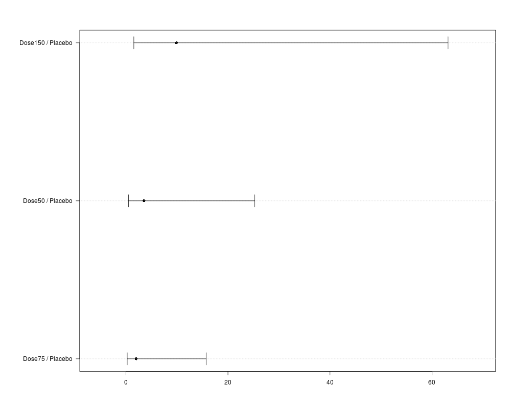
Simultaneous 95 percent-confidence intervals 
 for the odds ratio (OR) 
                  estimate  lower   upper
Dose150 / Placebo   9.9048 1.5551 63.0865
Dose50 / Placebo    3.5556 0.5008 25.2435
Dose75 / Placebo    2.0000 0.2547 15.7056
  
where the odds is defined: p(y)/(1-p(y)) 
  
> summary(ORlia)
Summary statistics: 
                            Dose150  Dose50  Dose75 Placebo
number of y                 13.0000  6.0000  4.0000  2.0000
number of trials            34.0000 33.0000 36.0000 34.0000
estimated probability of y   0.3824  0.1818  0.1111  0.0588

 Contrast matrix on the level of the logit link: 

	 Multiple Comparisons of Means: Dunnett Contrasts

                  Dose150 Dose50 Dose75 Placebo
Dose150 - Placebo       1      0      0      -1
Dose50 - Placebo        0      1      0      -1
Dose75 - Placebo        0      0      1      -1

 The estimated correlation matrix of the contrasts is: 
       [,1]   [,2]   [,3]
[1,] 1.0000 0.7652 0.7278
[2,] 0.7652 1.0000 0.6875
[3,] 0.7278 0.6875 1.0000

Simultaneous 95 percent-confidence intervals 
 for the odds ratio (OR) 
                  estimate  lower   upper
Dose150 / Placebo   9.9048 1.5551 63.0865
Dose50 / Placebo    3.5556 0.5008 25.2435
Dose75 / Placebo    2.0000 0.2547 15.7056
  
where the odds is defined: p(y)/(1-p(y)) 
  
> plot(ORlia)
> 
> # if data are available as table:
> 
> tab<-table(liarozole)
> tab
        Treatment
Improved Dose150 Dose50 Dose75 Placebo
       n      21     27     32      32
       y      13      6      4       2
> ORlia2<-binomORci(tab, success="y", type="Dunnett", base=4)
> ORlia2
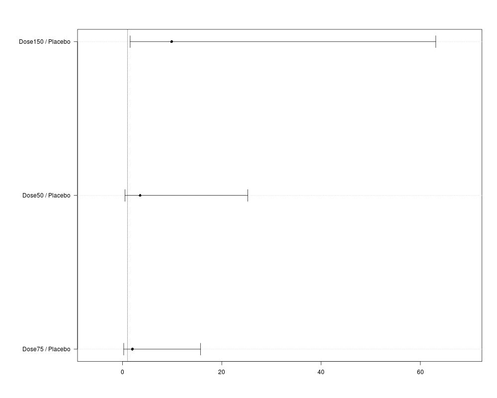
Simultaneous 95 percent-confidence intervals 
 for the odds ratio (OR) 
                  estimate  lower   upper
Dose150 / Placebo   9.9048 1.5551 63.0836
Dose50 / Placebo    3.5556 0.5008 25.2422
Dose75 / Placebo    2.0000 0.2547 15.7048
  
where the odds is defined: p(y)/(1-p(y)) 
  
> 
> plot(ORlia2, lines=1, lineslty=3)
> 
> 
> ############################
> 
> #  Performance for extreme cases
> 
> # method="GLM" (the default)
> 
> test1<-binomORci(x=c(0,1,5,20), n=c(20,20,20,20), names=c("A","B","C","D"))
> test1
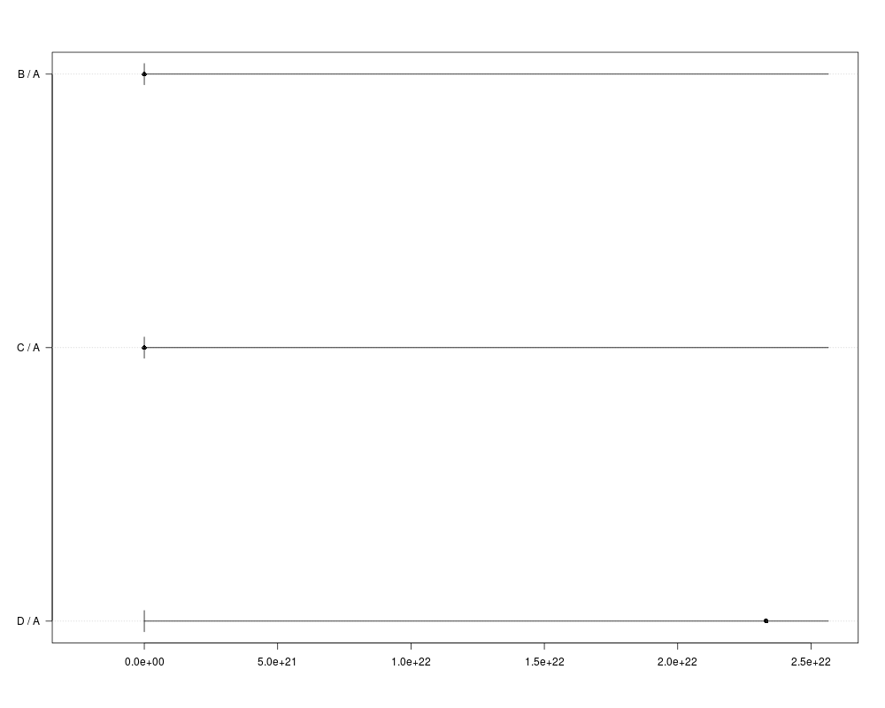
Simultaneous 95 percent-confidence intervals 
 for the odds ratio (OR) 
          estimate lower upper
B / A 8.037023e+09     0   Inf
C / A 5.090115e+10     0   Inf
D / A 2.331830e+22     0   Inf
  
where the odds is defined: p(success)/(1-p(success)) 
  
> plot(test1)
> 
> # adjusted Woolf interval
> 
> test2<-binomORci(x=c(0,1,5,20), n=c(20,20,20,20), names=c("A","B","C","D"), method="Woolf")
Warning message:
In restrictboundsOR(x = x, n = n, cmat = cmat, conf.int = conf.int) :
  0 occured in the data and the risk ratio might not be defined
> test2
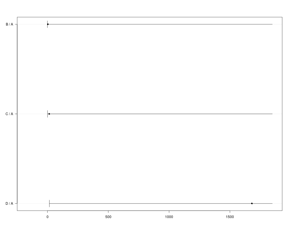
Simultaneous 95 percent-confidence intervals 
 for the odds ratio (OR) 
       estimate   lower upper
B / A    3.1538  0.0696   Inf
C / A   14.5484  0.4509   Inf
D / A 1681.0000 16.2056   Inf
  
where the odds is defined: p(success)/(1-p(success)) 
  
> plot(test2)
> 
> 
> 
> 
> 
> 
> dev.off()
null device 
          1 
>