R Graphical Manual

Browse All

Last data update: 2014.03.03

R: Simultaneous confidence intervals for contrasts of...

binomRDci

R Documentation

Simultaneous confidence intervals for contrasts of independent binomial proportions (in a oneway layout)

Description

Simultaneous asymptotic CI for contrasts of binomial proportions, assuming that standard normal approximation holds. The contrasts can be interpreted as differences of (weighted averages) of proportions (risk ratios).

Usage


binomRDci(x,...)

## Default S3 method:
binomRDci(x, n, names=NULL,
 type="Dunnett", cmat=NULL, method="Wald",
 alternative="two.sided", conf.level=0.95,
 dist="MVN", ...)

## S3 method for class 'formula'
binomRDci(formula, data,
 type="Dunnett", cmat=NULL, method="Wald",
 alternative="two.sided", conf.level=0.95,
 dist="MVN",...)

## S3 method for class 'table'
binomRDci(x, type="Dunnett",
 cmat=NULL, method="Wald", alternative="two.sided",
 conf.level=0.95, dist="MVN",...)

## S3 method for class 'matrix'
binomRDci(x, type="Dunnett",
 cmat=NULL, method="Wald", alternative="two.sided",
 conf.level=0.95, dist="MVN",...)

Arguments

`x`	a numeric vector, giving the number of successes in I independent samples, or an object of class `"table"`, representing the 2xk-table, or an object of class `"matrix"`, representing the 2xk-table
`n`	a numeric vector, giving the number of trials (i.e. the sample size) in each of the I groups (only required if `x` is a numeric vector, ignored otherwise)
`names`	an optional character string, giving the names of the groups/ sample in `x`, `n`; if not specified the possible names of x are taken as group names (ignored if `x` is a table or matrix)
`formula`	a two-sided formula of the style 'response ~ treatment', where 'response' should be a categorical variable with two levels, while treatment should be a factor specifying the treatment levels
`data`	a data.frame, containing the variables specified in formula
`type`	a character string, giving the name of a contrast method, as defined in `contrMat(multcomp)`; ignored if `cmat` is specified
`cmat`	a optional contrast matrix
`method`	a single character string, specifying the method for confidence interval construction; options are: `"Wald"`, `"ADD1"`, or `"ADD2"`
`alternative`	a single character string, one of "two.sided", "less", "greater"
`conf.level`	a single numeric value, simultaneous confidence level
`dist`	a character string, `"MVN"` invokes multiplicity adjustment via the multivariate normal distribution, `"N"` invokes use of quantiles of the univariate normal distribution
`...`	arguments to be passed to binomest, currently only `success` labelling the event which should be considered as success

Details

See the examples for different usages.

Value

A object of class "binomRDci", a list containing:

`conf.int`	a matrix with 2 columns: lower and upper confidence bounds, and M rows
`alternative`	character string, as input
`conf.level`	single numeric value, as input
`quantile`	the quantile used to construct the confidence intervals
`estimate`	a matrix with 1 column: containing the estimates of the contrasts
`x`	the observed number of successes in the treatment groups
`n`	the number of trials in the treatment groups
`p`	the estimated proportions in the treatment groups
`success`	a character string labelling the event considered as success
`names`	the group names
`method`	a character string, specifying the method of interval construction
`cmat`	the contrast matrix used

Note

Note, that all implemented methods are approximate only. The coverage probability of the intervals might seriously deviate from the nominal level for small sample sizes and extreme success probabilities. See the simulation results in Sill (2007) for details.

References

Schaarschmidt, F., Sill, M. and Hothorn, L.A. (2008): Approximate simultaneous confidence intervals for multiple contrasts of binomial proportions. Biometrical Journal 50, 782-792.

Background references:

The ideas underlying the "ADD1" and "ADD2" adjustment are described in:

Agresti, A. and Caffo, B.(2000): Simple and effective confidence intervals for proportions and differences of proportions result from adding two successes and two failures. American Statistician 54, p. 280-288.

And have been generalized for a single contrast of several proportions in:

Price, R.M. and Bonett, D.G. (2004): An improved confidence interval for a linear function of binomial proportions. Computational Statistics and Data Analysis 45, 449-456.

More detailed simulation results are available in:

Sill, M. (2007): Approximate simultaneous confidence intervals for multiple comparisons of binomial proportions. Master thesis, Institute of Biostatistics, Leibniz University Hannover.

Examples


###############################################################

### Example 1 Tables 1,7,8 in Schaarschmidt et al. (2008):  ###

###############################################################

# Number of patients under observation: 
n <- c(29, 24, 25, 24, 46)

# Number of patients with complete response:
cr <- c(7, 11, 10, 12, 21)

# (Optional) names for the treatments
dn <- c("0.3_1.0", "3", "10", "30", "90")

# Assume we aim to infer an increasing trend with increasing dosage,
# Using the changepoint contrasts (Table 7, Schaarschmidt et al., 2008)

# The results in Table 8 can be reproduced by calling:

binomRDci(n=n, x=cr, names=dn, alternative="greater",
 method="ADD2", type="Changepoint")

binomRDci(n=n, x=cr, names=dn, alternative="greater",
 method="ADD1", type="Changepoint")

binomRDci(n=n, x=cr, names=dn, alternative="greater", 
 method="Wald", type="Changepoint")

##############################################################

### Example 2, Tables 2,9,10 in Schaarschmidt et al. 2008  ###

##############################################################

# Data (Table 2)

# animals under risk
n<-c(30,30,30,30)

# animals showing cancer
cancer<-c(20,14,27,19)

# short names for the treatments
trtn<-c("HFaFi","LFaFi","HFaNFi","LFaNFi")


# User-defined contrast matrix (Table 9),
# columns of the contrast matrix 

cmat<-rbind(
"Fiber - No Fiber"=c( 0.5, 0.5,-0.5,-0.5),
"Low Fat - High Fat"=c(-0.5, 0.5,-0.5, 0.5),
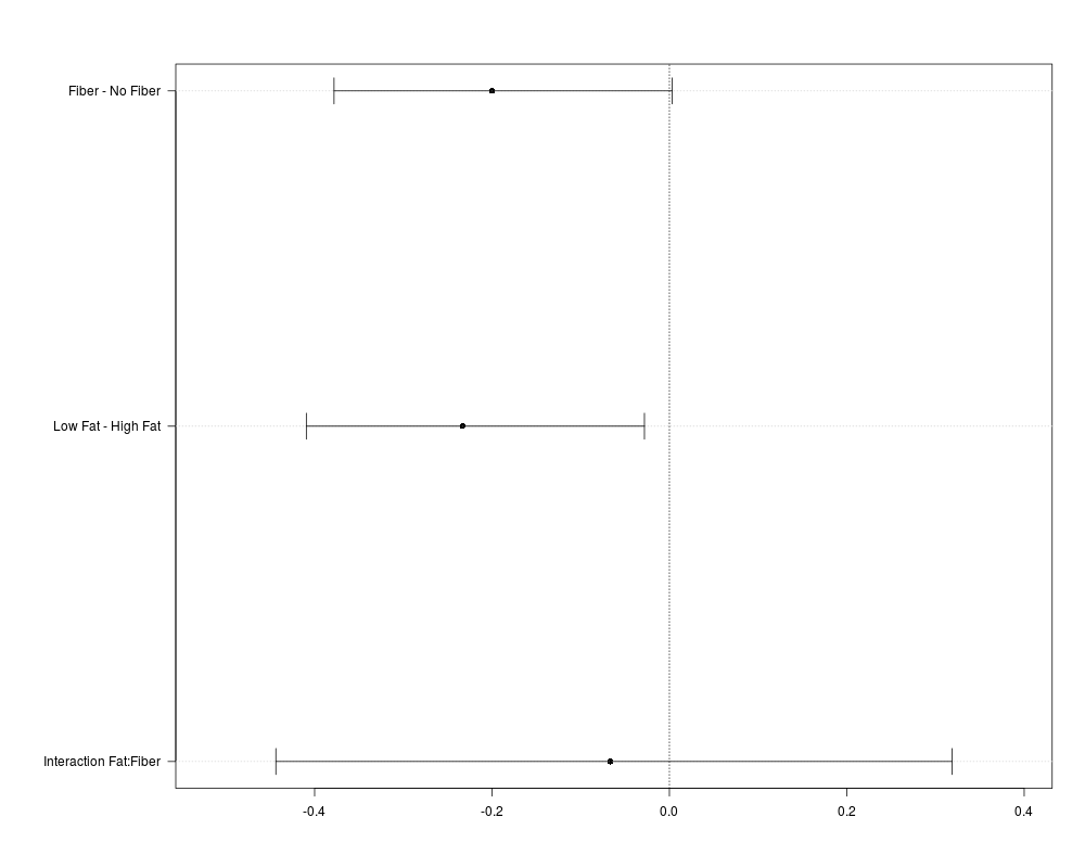
"Interaction Fat:Fiber"=c(   1,  -1,   -1,  1))

cmat

# The results in Table 10 can be reproduced by calling:

# simultaneous CI using the add-2 adjustment

sci<-binomRDci(x=cancer, n=n, names=trtn, method="ADD2",
 cmat=cmat, dist="MVN")

sci

# marginal CI using the basic Wald formula

ci<-binomRDci(x=cancer, n=n, names=trtn, method="Wald",
 cmat=cmat, dist="N")

ci


# check, whether the intended contrasts have been defined:

summary(sci)

# plot the result:

plot(sci, lines=0, lineslty=3)


##########################################


# In simple cases, counts of successes
# and number of trials can be just typed:

ntrials <- c(40,20,20,20)
xsuccesses <- c(1,2,2,4)
names(xsuccesses) <- LETTERS[1:4]
ex1D<-binomRDci(x=xsuccesses, n=ntrials, method="ADD1",
 type="Dunnett")
ex1D

ex1W<-binomRDci(x=xsuccesses, n=ntrials, method="ADD1",
 type="Williams", alternative="greater")
ex1W

# results can be plotted:
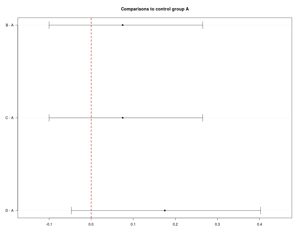
plot(ex1D, main="Comparisons to control group A", lines=0, linescol="red", lineslwd=2)

# summary gives a more detailed print out:
summary(ex1W)

# if data are represented as dichotomous variable
# in a data.frame one can make use of table:


#################################

data(liarozole)

head(liarozole)

binomRDci(Improved ~ Treatment, data=liarozole,
 type="Tukey")

# here, it might be important to define which level of the
# variable 'Improved' is to be considered as success

binomRDci(Improved ~ Treatment, data=liarozole,
 type="Dunnett", success="y", base=4)

# If data are available as a named kx2-contigency table:

tab<-table(liarozole)
tab

# Comparison to the control group "Placebo",
# which is the fourth group in alpha-numeric order:

CIs<-binomRDci(tab, type="Dunnett", success="y", base=4)

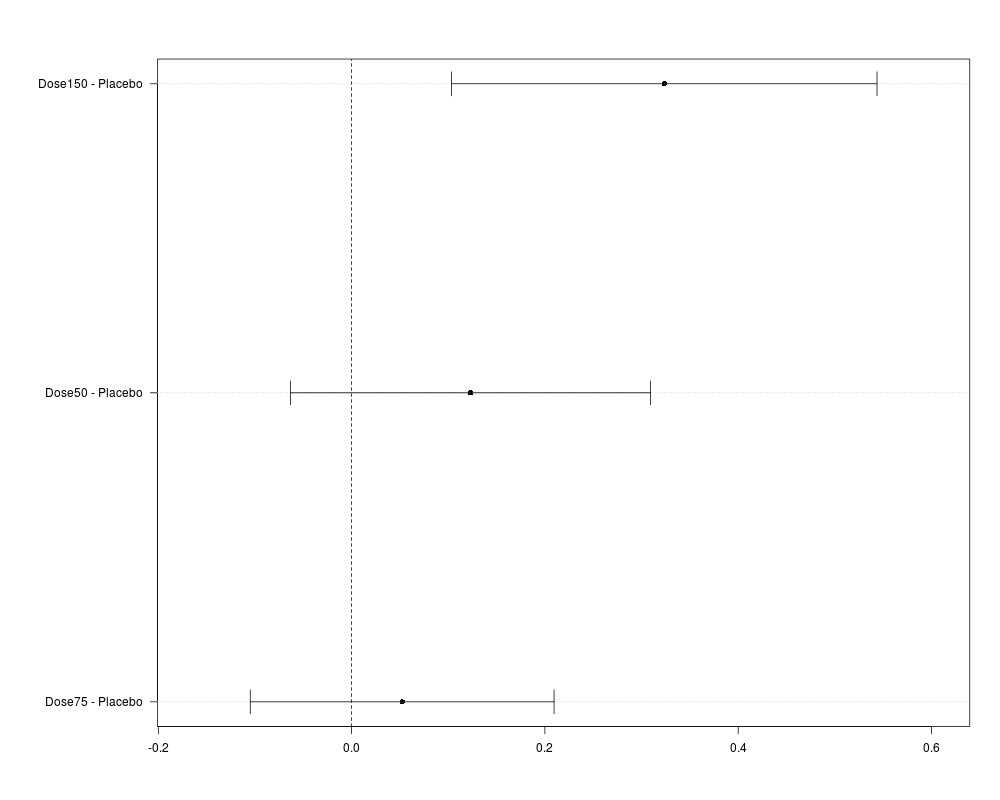
plot(CIs, lines=0)

Results


R version 3.3.1 (2016-06-21) -- "Bug in Your Hair"
Copyright (C) 2016 The R Foundation for Statistical Computing
Platform: x86_64-pc-linux-gnu (64-bit)

R is free software and comes with ABSOLUTELY NO WARRANTY.
You are welcome to redistribute it under certain conditions.
Type 'license()' or 'licence()' for distribution details.

R is a collaborative project with many contributors.
Type 'contributors()' for more information and
'citation()' on how to cite R or R packages in publications.

Type 'demo()' for some demos, 'help()' for on-line help, or
'help.start()' for an HTML browser interface to help.
Type 'q()' to quit R.

> library(MCPAN)
> png(filename="/home/ddbj/snapshot/RGM3/R_CC/result/MCPAN/binomRDci.Rd_%03d_medium.png", width=480, height=480)
> ### Name: binomRDci
> ### Title: Simultaneous confidence intervals for contrasts of independent
> ###   binomial proportions (in a oneway layout)
> ### Aliases: binomRDci binomRDci.default binomRDci.table binomRDci.matrix
> ###   binomRDci.formula
> ### Keywords: htest
> 
> ### ** Examples
> 
> 
> ###############################################################
> 
> ### Example 1 Tables 1,7,8 in Schaarschmidt et al. (2008):  ###
> 
> ###############################################################
> 
> # Number of patients under observation: 
> n <- c(29, 24, 25, 24, 46)
> 
> # Number of patients with complete response:
> cr <- c(7, 11, 10, 12, 21)
> 
> # (Optional) names for the treatments
> dn <- c("0.3_1.0", "3", "10", "30", "90")
> 
> # Assume we aim to infer an increasing trend with increasing dosage,
> # Using the changepoint contrasts (Table 7, Schaarschmidt et al., 2008)
> 
> # The results in Table 8 can be reproduced by calling:
> 
> binomRDci(n=n, x=cr, names=dn, alternative="greater",
+  method="ADD2", type="Changepoint")
Simultaneous 95 percent Add-2 -confidence intervals 
 for the difference of proportions (RD) 
    estimate   lower upper
C 1   0.2124  0.0063   Inf
C 2   0.1130 -0.0635   Inf
C 3   0.1125 -0.0617   Inf
C 4   0.0644 -0.1230   Inf
  
where proportions are the probabilities to observe success 
  
> 
> binomRDci(n=n, x=cr, names=dn, alternative="greater",
+  method="ADD1", type="Changepoint")
Simultaneous 95 percent Add-1 -confidence intervals 
 for the difference of proportions (RD) 
    estimate   lower upper
C 1   0.2124  0.0110   Inf
C 2   0.1130 -0.0624   Inf
C 3   0.1125 -0.0604   Inf
C 4   0.0644 -0.1230   Inf
  
where proportions are the probabilities to observe success 
  
> 
> binomRDci(n=n, x=cr, names=dn, alternative="greater", 
+  method="Wald", type="Changepoint")
Simultaneous 95 percent Wald -confidence intervals 
 for the difference of proportions (RD) 
    estimate   lower upper
C 1   0.2124  0.0169   Inf
C 2   0.1130 -0.0605   Inf
C 3   0.1125 -0.0582   Inf
C 4   0.0644 -0.1221   Inf
  
where proportions are the probabilities to observe success 
  
> 
> ##############################################################
> 
> ### Example 2, Tables 2,9,10 in Schaarschmidt et al. 2008  ###
> 
> ##############################################################
> 
> # Data (Table 2)
> 
> # animals under risk
> n<-c(30,30,30,30)
> 
> # animals showing cancer
> cancer<-c(20,14,27,19)
> 
> # short names for the treatments
> trtn<-c("HFaFi","LFaFi","HFaNFi","LFaNFi")
> 
> 
> # User-defined contrast matrix (Table 9),
> # columns of the contrast matrix 
> 
> cmat<-rbind(
+ "Fiber - No Fiber"=c( 0.5, 0.5,-0.5,-0.5),
+ "Low Fat - High Fat"=c(-0.5, 0.5,-0.5, 0.5),
+ "Interaction Fat:Fiber"=c(   1,  -1,   -1,  1))
> 
> cmat
                      [,1] [,2] [,3] [,4]
Fiber - No Fiber       0.5  0.5 -0.5 -0.5
Low Fat - High Fat    -0.5  0.5 -0.5  0.5
Interaction Fat:Fiber  1.0 -1.0 -1.0  1.0
> 
> # The results in Table 10 can be reproduced by calling:
> 
> # simultaneous CI using the add-2 adjustment
> 
> sci<-binomRDci(x=cancer, n=n, names=trtn, method="ADD2",
+  cmat=cmat, dist="MVN")
> 
> sci
Simultaneous 95 percent Add-2 -confidence intervals 
 for the difference of proportions (RD) 
                      estimate   lower   upper
Fiber - No Fiber       -0.2000 -0.3782  0.0032
Low Fat - High Fat     -0.2333 -0.4094 -0.0281
Interaction Fat:Fiber  -0.0667 -0.4439  0.3189
  
where proportions are the probabilities to observe success 
  
> 
> # marginal CI using the basic Wald formula
> 
> ci<-binomRDci(x=cancer, n=n, names=trtn, method="Wald",
+  cmat=cmat, dist="N")
> 
> ci
Local 95 percent Wald -confidence intervals 
 for the difference of proportions (RD) 
                      estimate   lower   upper
Fiber - No Fiber       -0.2000 -0.3594 -0.0406
Low Fat - High Fat     -0.2333 -0.3927 -0.0740
Interaction Fat:Fiber  -0.0667 -0.3854  0.2521
  
where proportions are the probabilities to observe success 
  
> 
> 
> # check, whether the intended contrasts have been defined:
> 
> summary(sci)
Summary statistics: 
                                HFaFi   LFaFi HFaNFi  LFaNFi
number of successes           20.0000 14.0000   27.0 19.0000
number of trials              30.0000 30.0000   30.0 30.0000
estimated success probability  0.6667  0.4667    0.9  0.6333

 Contrast matrix: 
                      HFaFi LFaFi HFaNFi LFaNFi
Fiber - No Fiber        0.5   0.5   -0.5   -0.5
Low Fat - High Fat     -0.5   0.5   -0.5    0.5
Interaction Fat:Fiber   1.0  -1.0   -1.0    1.0

 The estimated correlation matrix of the contrasts is: 
        [,1]    [,2]    [,3]
[1,]  1.0000 -0.1241 -0.1814
[2,] -0.1241  1.0000 -0.1599
[3,] -0.1814 -0.1599  1.0000

Simultaneous 95 percent Add-2 -confidence intervals 
 for the difference of proportions (RD) 
                      estimate   lower   upper
Fiber - No Fiber       -0.2000 -0.3782  0.0032
Low Fat - High Fat     -0.2333 -0.4094 -0.0281
Interaction Fat:Fiber  -0.0667 -0.4439  0.3189
  
where proportions are the probabilities to observe success 
  
> 
> # plot the result:
> 
> plot(sci, lines=0, lineslty=3)
> 
> 
> ##########################################
> 
> 
> # In simple cases, counts of successes
> # and number of trials can be just typed:
> 
> ntrials <- c(40,20,20,20)
> xsuccesses <- c(1,2,2,4)
> names(xsuccesses) <- LETTERS[1:4]
> ex1D<-binomRDci(x=xsuccesses, n=ntrials, method="ADD1",
+  type="Dunnett")
> ex1D
Simultaneous 95 percent Add-1 -confidence intervals 
 for the difference of proportions (RD) 
      estimate  lower  upper
B - A    0.075 -0.100 0.2650
C - A    0.075 -0.100 0.2650
D - A    0.175 -0.047 0.4024
  
where proportions are the probabilities to observe success 
  
> 
> ex1W<-binomRDci(x=xsuccesses, n=ntrials, method="ADD1",
+  type="Williams", alternative="greater")
> ex1W
Simultaneous 95 percent Add-1 -confidence intervals 
 for the difference of proportions (RD) 
    estimate   lower upper
C 1   0.1750 -0.0051   Inf
C 2   0.1250  0.0056   Inf
C 3   0.1083  0.0104   Inf
  
where proportions are the probabilities to observe success 
  
> 
> # results can be plotted:
> plot(ex1D, main="Comparisons to control group A", lines=0, linescol="red", lineslwd=2)
> 
> # summary gives a more detailed print out:
> summary(ex1W)
Summary statistics: 
                                   A    B    C    D
number of successes            1.000  2.0  2.0  4.0
number of trials              40.000 20.0 20.0 20.0
estimated success probability  0.025  0.1  0.1  0.2

 Contrast matrix: 

	 Multiple Comparisons of Means: Williams Contrasts

     A      B      C      D
C 1 -1 0.0000 0.0000 1.0000
C 2 -1 0.0000 0.5000 0.5000
C 3 -1 0.3333 0.3333 0.3333

 The estimated correlation matrix of the contrasts is: 
       [,1]   [,2]   [,3]
[1,] 1.0000 0.8057 0.7010
[2,] 0.8057 1.0000 0.8829
[3,] 0.7010 0.8829 1.0000

Simultaneous 95 percent Add-1 -confidence intervals 
 for the difference of proportions (RD) 
    estimate   lower upper
C 1   0.1750 -0.0051   Inf
C 2   0.1250  0.0056   Inf
C 3   0.1083  0.0104   Inf
  
where proportions are the probabilities to observe success 
  
> 
> # if data are represented as dichotomous variable
> # in a data.frame one can make use of table:
> 
> 
> #################################
> 
> data(liarozole)
> 
> head(liarozole)
  Improved Treatment
1        y   Placebo
2        y   Placebo
3        n   Placebo
4        n   Placebo
5        n   Placebo
6        n   Placebo
> 
> binomRDci(Improved ~ Treatment, data=liarozole,
+  type="Tukey")
Simultaneous 95 percent Wald -confidence intervals 
 for the difference of proportions (RD) 
                  estimate   lower  upper
Dose50 - Dose150    0.2005 -0.0728 0.4739
Dose75 - Dose150    0.2712  0.0198 0.5227
Placebo - Dose150   0.3235  0.0870 0.5601
Dose75 - Dose50     0.0707 -0.1468 0.2882
Placebo - Dose50    0.1230 -0.0771 0.3231
Placebo - Dose75    0.0523 -0.1166 0.2212
  
where proportions are the probabilities to observe n 
  
> 
> # here, it might be important to define which level of the
> # variable 'Improved' is to be considered as success
> 
> binomRDci(Improved ~ Treatment, data=liarozole,
+  type="Dunnett", success="y", base=4)
Simultaneous 95 percent Wald -confidence intervals 
 for the difference of proportions (RD) 
                  estimate   lower   upper
Dose50 - Dose150   -0.2005 -0.4461  0.0450
Dose75 - Dose150   -0.2712 -0.4971 -0.0454
Placebo - Dose150  -0.3235 -0.5360 -0.1111
  
where proportions are the probabilities to observe y 
  
> 
> # If data are available as a named kx2-contigency table:
> 
> tab<-table(liarozole)
> tab
        Treatment
Improved Dose150 Dose50 Dose75 Placebo
       n      21     27     32      32
       y      13      6      4       2
> 
> # Comparison to the control group "Placebo",
> # which is the fourth group in alpha-numeric order:
> 
> CIs<-binomRDci(tab, type="Dunnett", success="y", base=4)
> 
> plot(CIs, lines=0)
> 
> 
> 
> 
> 
> 
> dev.off()
null device 
          1 
>