R Graphical Manual

Browse All

Last data update: 2014.03.03

R: Simultaneous confidence intervals for contrasts of...

poly3ci

R Documentation

Simultaneous confidence intervals for contrasts of poly-3-adjusted tumour rates

Description

Function to calculate simultaneous confidence intervals for several contrasts of poly-3-adjusted tumour rates in a oneway layout. Assuming a data situation as in Peddada(2005) or Bailer and Portier (1988). Simultaneous asymptotic CI for contrasts of tumour rates, assuming that standard normal approximation holds.

Usage

poly3ci(time, status, f, type = "Dunnett",
 cmat = NULL, method = "BP", alternative = "two.sided",
 conf.level = 0.95, dist="MVN", k=3, ...)

Arguments

`time`	a numeric vector of times of death of the individuals
`status`	a logical (or numeric, consisting of 0,1 only) vector giving the tumour status at time of death of each individual, where TRUE (1) = tumour present, FALSE (0) = no tumour present
`f`	a factor, giving the classification variable
`type`	a character string, giving the name of a contrast method, as defined in `contrMat(multcomp)`
`cmat`	a optional contrast matrix
`method`	a single charcter string, specifying the method for adjustment, with options: "BP" (Bailer Portier: assuming poly-3-adjusted rates are binomial variables), "BW" (Bieler, Williams: delta method as in Bieler and Williams (1993)) "ADD1" (as Bailer Portier, including an add1-adjustment on the raw tumour rates) "ADD2" (as Bailer Portier, including an add2-adjustment on the raw tumour rates following Agresti and Caffo (2000) for binomials)
`alternative`	a single character string
`conf.level`	a single numeric value, simultaneous confidence level
`dist`	a character string, `"MVN"` invokes multiplicity adjustment via the multivariate normal distribution, `"N"` invokes use of quantiles of the univariate normal distribution
`k`	the exponent to calculate survival adjusted proportions, default is k=3
`...`	further arguments to be passed; currently only base, to be passed to `contrMat` to choose the control group with `type="Dunnett"`

Value

A object of class "poly3ci", a list containing:

`conf.int`	a matrix with 2 columns: lower and upper confidence bounds, and M rows
`alternative`	character string, as input
`conf.level`	single numeric value, as input
`quantile`	the quantile used to construct the CIs
`estimate`	a numeric vector with the point estimates of the contrasts
`time`	as input
`status`	as input
`f`	as input
`method`	as input
`cmat`	as input, with colnames= factor levels of f
`sample.est`	a list containing sample estimates

Note

Please note that all methods here described are only approximative, and might violate the nominal level in certain situations. Please note further that appropriateness of the point estimates, and consequently of tests and confidence intervals is based on the assumptions in Bailer and Portier (1988), which might be a matter of controversies.

Author(s)

Frank Schaarschmidt

References

The implemented methodology is described in:

Schaarschmidt, F., Sill, M., and Hothorn, L.A. (2008): Approximate Simultaneous confidence intervals for multiple contrasts of binomial proportions. Biometrical Journal 50, 782-792.

Background references are:

Assumption for poly-3-adjustment: Bailer, J.A. and Portier, C.J. (1988): Effects of treatment-induced mortality and tumor-induced mortality on tests for carcinogenicity in small samples. Biometrics 44, 417-431.

Peddada, S.D., Dinse, G.E., and Haseman, J.K. (2005): A survival-adjusted quantal response test for comparing tumor incidence rates. Applied Statistics 54, 51-61.

Bieler, G.S. and Williams, R.L. (1993): Ratio estimates, the Delta Method, and quantal response tests for increased carcinogenicity. Biometrics 49, 793-801.

Statistical procedures and characterization of the coverage probabilities are described in: Sill, M. (2007): Approximate simultaneous confidence intervals for multiple comparisons of binomial proportions. Master thesis, Institute of Biostatistics, Leibniz University Hannover.

Examples


#############################################################

### Methyleugenol example in Schaarschmidt et al. (2008) ####

#############################################################

# load the data:

data(methyl)

# The results in Table 5 (Schaarschmidt et al. 2008) can be
# reproduced by calling:


methylW<-poly3ci(time=methyl$death, status=methyl$tumour,
 f=methyl$group, type = "Williams", method = "ADD1", alternative="greater" )

methylW


methylWT<-poly3test(time=methyl$death, status=methyl$tumour,
 f=methyl$group, type = "Williams", method = "ADD1", alternative="greater" )

methylWT


plot(methylW, main="Simultaneous CI for \n Poly-3-adjusted tumour rates")

# The results in Table 6 can be reproduced by calling:

methylD<-poly3ci(time=methyl$death, status=methyl$tumour,
 f=methyl$group, type = "Dunnett", method = "ADD1", alternative="greater" )

methylD

methylDT<-poly3test(time=methyl$death, status=methyl$tumour,
 f=methyl$group, type = "Dunnett", method = "ADD1", alternative="greater" )

methylDT


plot(methylD, main="Simultaneous CI for Poly-3-adjusted tumour rates", cex.main=0.7)


############################################################


# unadjusted CI

methylD1<-poly3ci(time=methyl$death, status=methyl$tumour,
 f=methyl$group, type = "Dunnett", method = "ADD1", dist="N" )

methylD1

plot(methylD1, main="Local CI for Poly-3-adjusted tumour rates")

Results


R version 3.3.1 (2016-06-21) -- "Bug in Your Hair"
Copyright (C) 2016 The R Foundation for Statistical Computing
Platform: x86_64-pc-linux-gnu (64-bit)

R is free software and comes with ABSOLUTELY NO WARRANTY.
You are welcome to redistribute it under certain conditions.
Type 'license()' or 'licence()' for distribution details.

R is a collaborative project with many contributors.
Type 'contributors()' for more information and
'citation()' on how to cite R or R packages in publications.

Type 'demo()' for some demos, 'help()' for on-line help, or
'help.start()' for an HTML browser interface to help.
Type 'q()' to quit R.

> library(MCPAN)
> png(filename="/home/ddbj/snapshot/RGM3/R_CC/result/MCPAN/poly3ci.Rd_%03d_medium.png", width=480, height=480)
> ### Name: poly3ci
> ### Title: Simultaneous confidence intervals for contrasts of
> ###   poly-3-adjusted tumour rates
> ### Aliases: poly3ci
> ### Keywords: htest
> 
> ### ** Examples
> 
> 
> #############################################################
> 
> ### Methyleugenol example in Schaarschmidt et al. (2008) ####
> 
> #############################################################
> 
> # load the data:
> 
> data(methyl)
> 
> # The results in Table 5 (Schaarschmidt et al. 2008) can be
> # reproduced by calling:
> 
> 
> methylW<-poly3ci(time=methyl$death, status=methyl$tumour,
+  f=methyl$group, type = "Williams", method = "ADD1", alternative="greater" )
> 
> methylW
Sample estimates, using poly- 3 -adjustment 
                        0       1       2       3
x                  1.0000  9.0000  8.0000  5.0000
n                 50.0000 50.0000 50.0000 50.0000
adjusted n        41.4046 40.3112 38.7444 32.6983
adjusted estimate  0.0242  0.2233  0.2065  0.1529
  
Contrast matrix: 

	 Multiple Comparisons of Means: Williams Contrasts

     0      1      2      3
C 1 -1 0.0000 0.0000 1.0000
C 2 -1 0.0000 0.5000 0.5000
C 3 -1 0.3333 0.3333 0.3333
  
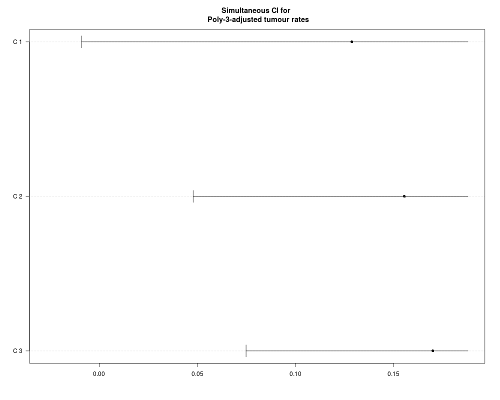
Simultaneous 95 percent confidence intervals using Add-1 variance estimators: 
    estimate   lower upper
C 1   0.1288 -0.0088   Inf
C 2   0.1555  0.0480   Inf
C 3   0.1701  0.0750   Inf
  
> 
> 
> methylWT<-poly3test(time=methyl$death, status=methyl$tumour,
+  f=methyl$group, type = "Williams", method = "ADD1", alternative="greater" )
> 
> methylWT
Sample estimates using poly- 3 -adjustment 
                        0       1       2       3
x                  1.0000  9.0000  8.0000  5.0000
n                 50.0000 50.0000 50.0000 50.0000
adjusted n        41.4046 40.3112 38.7444 32.6983
adjusted estimate  0.0242  0.2233  0.2065  0.1529
  
Contrast matrix: 

	 Multiple Comparisons of Means: Williams Contrasts

     0      1      2      3
C 1 -1 0.0000 0.0000 1.0000
C 2 -1 0.0000 0.5000 0.5000
C 3 -1 0.3333 0.3333 0.3333
  
Union-Intersection test using Add-1  variance estimator: 
P-value of the maximum test: 
[1] 4e-04
  
    estimate testat p.val.adj
C 1   0.1288 1.8342    0.0657
C 2   0.1555 2.8563    0.0051
C 3   0.1701 3.5588    0.0004
  
> 
> 
> plot(methylW, main="Simultaneous CI for \n Poly-3-adjusted tumour rates")
> 
> # The results in Table 6 can be reproduced by calling:
> 
> methylD<-poly3ci(time=methyl$death, status=methyl$tumour,
+  f=methyl$group, type = "Dunnett", method = "ADD1", alternative="greater" )
> 
> methylD
Sample estimates, using poly- 3 -adjustment 
                        0       1       2       3
x                  1.0000  9.0000  8.0000  5.0000
n                 50.0000 50.0000 50.0000 50.0000
adjusted n        41.4046 40.3112 38.7444 32.6983
adjusted estimate  0.0242  0.2233  0.2065  0.1529
  
Contrast matrix: 

	 Multiple Comparisons of Means: Dunnett Contrasts

       0 1 2 3
1 - 0 -1 1 0 0
2 - 0 -1 0 1 0
3 - 0 -1 0 0 1
  
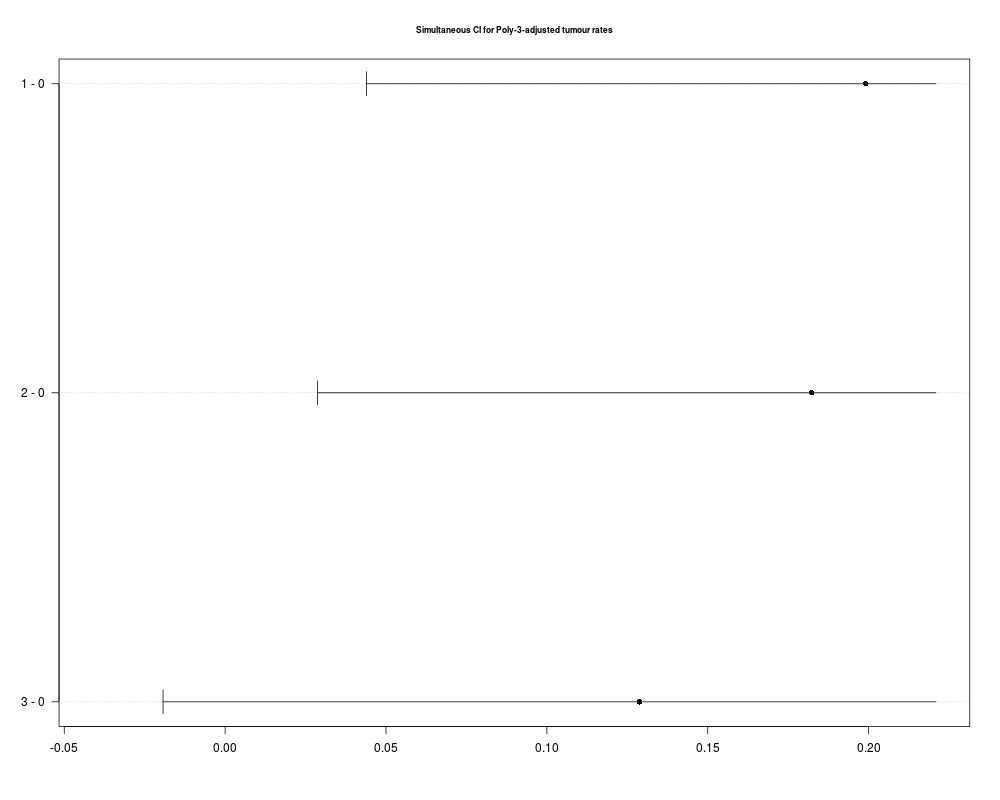
Simultaneous 95 percent confidence intervals using Add-1 variance estimators: 
      estimate   lower upper
1 - 0   0.1991  0.0439   Inf
2 - 0   0.1823  0.0287   Inf
3 - 0   0.1288 -0.0193   Inf
  
> 
> methylDT<-poly3test(time=methyl$death, status=methyl$tumour,
+  f=methyl$group, type = "Dunnett", method = "ADD1", alternative="greater" )
> 
> methylDT
Sample estimates using poly- 3 -adjustment 
                        0       1       2       3
x                  1.0000  9.0000  8.0000  5.0000
n                 50.0000 50.0000 50.0000 50.0000
adjusted n        41.4046 40.3112 38.7444 32.6983
adjusted estimate  0.0242  0.2233  0.2065  0.1529
  
Contrast matrix: 

	 Multiple Comparisons of Means: Dunnett Contrasts

       0 1 2 3
1 - 0 -1 1 0 0
2 - 0 -1 0 1 0
3 - 0 -1 0 0 1
  
Union-Intersection test using Add-1  variance estimator: 
P-value of the maximum test: 
[1] 0.0095
  
      estimate testat p.val.adj
1 - 0   0.1991 2.7271    0.0095
2 - 0   0.1823 2.5155    0.0175
3 - 0   0.1288 1.8342    0.0934
  
> 
> 
> plot(methylD, main="Simultaneous CI for Poly-3-adjusted tumour rates", cex.main=0.7)
> 
> 
> ############################################################
> 
> 
> # unadjusted CI
> 
> methylD1<-poly3ci(time=methyl$death, status=methyl$tumour,
+  f=methyl$group, type = "Dunnett", method = "ADD1", dist="N" )
> 
> methylD1
Sample estimates, using poly- 3 -adjustment 
                        0       1       2       3
x                  1.0000  9.0000  8.0000  5.0000
n                 50.0000 50.0000 50.0000 50.0000
adjusted n        41.4046 40.3112 38.7444 32.6983
adjusted estimate  0.0242  0.2233  0.2065  0.1529
  
Contrast matrix: 

	 Multiple Comparisons of Means: Dunnett Contrasts

       0 1 2 3
1 - 0 -1 1 0 0
2 - 0 -1 0 1 0
3 - 0 -1 0 0 1
  
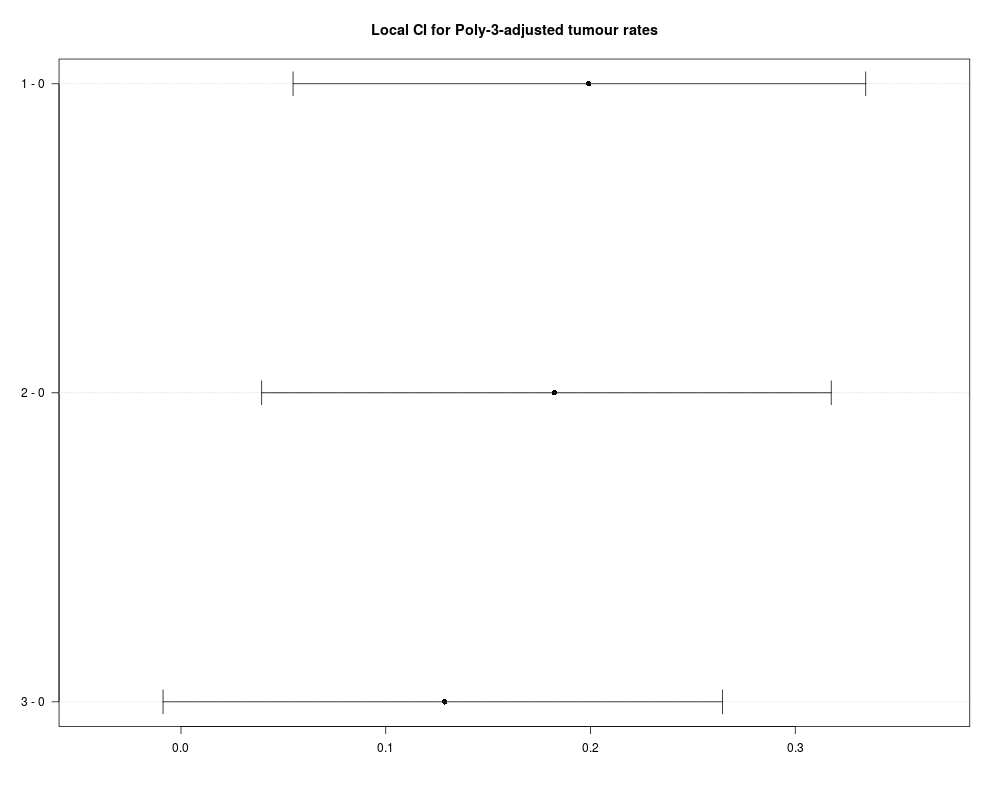
Local 95 percent confidence intervals using Add-1 variance estimators: 
      estimate   lower  upper
1 - 0   0.1991  0.0547 0.3344
2 - 0   0.1823  0.0394 0.3176
3 - 0   0.1288 -0.0088 0.2644
  
> 
> plot(methylD1, main="Local CI for Poly-3-adjusted tumour rates")
> 
> 
> 
> 
> 
> 
> dev.off()
null device 
          1 
>