R Graphical Manual

Browse All

Last data update: 2014.03.03

R: Perform MCPMod analysis of a data set

MCPMod

R Documentation

Perform MCPMod analysis of a data set

Description

Tests for a dose-response effect with a model-based multiple contrast test and estimates a target dose with regression techniques. For details see Bretz et al. (2005) or the enclosed vignette, available via the command vignette("MCPMod").

Usage

MCPMod(data, models = NULL, contMat = NULL, critV = NULL, resp = "resp",
       dose = "dose", off = NULL, scal = NULL, alpha = 0.025, 
       twoSide = FALSE, selModel = c("maxT", "AIC", "BIC", "aveAIC", 
       "aveBIC"), doseEst = c("MED2", "MED1", "MED3", "ED"), std = TRUE,
       start = NULL, uModPars = NULL, addArgs = NULL, dePar = NULL,
       clinRel = NULL, lenDose = 101, pW = NULL,
       control = list(maxiter = 100, tol = 1e-06, minFactor = 1/1024),
       signTtest = 1, pVal = FALSE, testOnly = FALSE,
       mvtcontrol = mvtnorm.control(), na.action = na.fail, uGrad = NULL)

Arguments

`data`	Data frame containing the dose and the response data. The code assumes the columns to be named "dose" and "resp". Other names can be handed over via the `dose` and `resp` argument see below.
`models`	A list specifying the candidate models. The names of the list entries should be equal to the names of the model functions. The list entries should be equal to the guesstimates. See the Examples (ii) for details on this topic. If the `contMat` argument is specified, this argument is ignored, see Examples (iv).
`contMat`	Optional matrix containing the optimal contrasts in the columns. The names of the columns should be equal to the underlying model function names. If specified the code does not calculate the optimal contrasts.
`critV`	Optional numeric specifying the critical value to be used in the multiple contrast test.
`resp`	Character string giving the name of the response column for the data frame specified in `data` (default: "resp").
`dose`	Character string giving the name of the dose column for the data frame specified in `data` (default: "dose").
`off`	Fixed offset parameter needed when the linear in log model is used. See also documentation of the linear in log model: `linlog`. When `off = NULL` by default (maximum dose)*0.1 is used for `off`.
`scal`	Fixed scale parameter needed when the beta model is used. See also documentation of the beta model: `betaMod`. When `scal = NULL` by default (maximum dose)*1.2 is used for `scal`.
`alpha`	Level of significance for the multiple contrast test (defaults to 0.025)
`twoSide`	Optional logical value deterimining whether two-sided or one-sided testing should be performed. Defaults to FALSE, so one-sided testing.
`selModel`	Optional character vector specifying the model selection criterion for dose estimation. Possible values are "maxT": Selects the model corresponding to the largest t-statistic (this is the default). "AIC": Selects model with smallest AIC "BIC": Selects model with smallest BIC "aveAIC": Uses a weighted average of the models corresponding to the significant contrasts. The model weights are chosen by the formula: wi = exp(-0.5AICi)/sum(exp(-0.5AICi)). See Buckland et al. (1997) for details. "aveBIC": Same as "aveAIC", but the BIC is used to calculate the model weights.
`doseEst`	Determines which dose to estimate and which dose estimator to use, possible values are "MED2", "MED1", "MED3" and "ED". See Bretz et al. (2005) for the definition of MED1-MED3. If ED is specified, the dose that gives a pre-specified percentage of the maximum effect is returned.
`std`	Optional logical value determining, whether standardized versions should be assumed for calculation of the optimal contrasts. If FALSE all model parameters need to be specified in the models argument (also location and scale parameters).
`start`	List containing starting values for the nls fitting algorithm. The names of the list elements need to be equal to the names of the model functions. The names of the starting vector should equal the corresponding names for the model parameters. For built-in models starting values need to be provided only for the non-linear parameters. In case of a user model (not built in) starting values for the all parameters need to be supplied. (see Examples (iii) for details).
`uModPars`	Optional character vector with names/expressions of user-defined model parameters (names(start) used by default).
`addArgs`	Optional character vector with names of additional arguments (variables) to user-defined model.
`dePar`	Numeric, defining parameter used for dose estimators. For the MED-type estimators `dePar` determines the confidence level gamma used in the estimator. The used confidence level is given by `1-2*dePar`. The default for `dePar` for MED-type estimators is 0.1. For ED-type estimators `dePar` determines which effective dose is estimated. Specifying 0.95 for example results in an estimate of the ED95. If the ED estimator is used the default for `dePar` is 0.5.
`clinRel`	Numeric specifying the clinical relevance threshold.
`lenDose`	Numeric vector specifying the number of points in the dose-range to search for the dose estimate, defaults to 101.
`pW`	Optional vector specifying prior weights for the different models. Should be a named vector with names matching the names of the models list.
`control`	List of parameters to be used in the calls to the `nls` function. See also `nls.control` function.
`signTtest`	Optional numeric vector multiplied with the test statistics.
`pVal`	Optional logical determining whether p-values should be calculated, defaults to FALSE. If the critical value is supplied, p-values will not be calculated.
`testOnly`	Logical value determining, whether only the multiple comparisons test should be performed. See Examples (v) below.
`mvtcontrol`	A list specifying additional control parameters for the `qmvt` and `pmvt` calls in the code, see also `mvtnorm.control` for details.
`na.action`	A function which indicates what should happen when the data contain NAs.
`uGrad`	Function to return the gradient of a user defined model, see Examples (iii) below.

Details

This function performs the multiple comparisons and modelling (MCPMod) procedure presented in Bretz et al. (2005). The method consists of two steps:
(i) MCP step: The function calculates the optimal contrasts (if not supplied) and the contrast test statistics. In the calculation of the critical value and p-values multiplicity is taken into account.
(ii) Modelling step: If there is at least one significant contrast, one model or a combination of models is chosen (depending on the selModel argument) for dose estimation. In case of non-convergence of certain non-linear models the remaining significant models are used. Finally the target dose is estimated.

Built in models are the linear, linear in log, emax, sigmoid emax, logistic, exponential, quadratic and beta model (for their definitions see their help files or Bretz et al. (2005), Pinheiro et al. (2006)). Users may hand over their own model functions for details have a look at the Example (iii).

Value

An object of class MCPMod, with the following entries:

`signf`	Logical indicating, whether multiple contrast test is significant
`model1`	Model with largest contrast test statistic
`model2`	Model(s) used for estimation of target doses
`input`	A list with entries equal to the input parameters for the function: `models`, `resp`, `dose`, `off`, `scal`, `alpha`, `twoSide`, first entry of `selModel`, `doseEst`, `std`, `dePar`, `uModArgs`, `addArgs`, `start`, `uGrad`, `clinRel`, `lenDose`, `signTtest`, `pVal`, `testOnly`
`data`	The data set.
`contMat`	The contrast matrix.
`corMat`	The correlation matrix.
`cVal`	The critical value for the multiple contrast test.
`tStat`	The contrast test-statistics. If 'pVal=TRUE' the p-values are also attached.
`fm`	List containing the dose-response model(s) used for dose-estimation. WARNING: The model fitting is for computational efficiency done based on the group means and for positive non-linear parameters (e.g. the ED50 parameter in the Emax model) the estimate in `fm` is on log scale. The summary.MCPMod method shows the parameters on their original scale. Hence some care is hence needed when extracting the fitted model objects from `fm` (in particular when interest is in standard deviations of predictions, parameter estimates...).
`tdose`	Estimated target dose, in case of model averaging the dose estimates under the individual models are attached.

Note: If testOnly=TRUE, or no model is significant, the object does not contain fm and tdose entries

References

Bornkamp B., Pinheiro J. C., and Bretz, F. (2009). MCPMod: An R Package for the Design and Analysis of Dose-Finding Studies, Journal of Statistical Software, 29(7), 1–23

Bretz, F., Pinheiro, J. C., and Branson, M. (2005), Combining multiple comparisons and modeling techniques in dose-response studies, Biometrics, 61, 738–748

Pinheiro, J. C., Bornkamp, B., and Bretz, F. (2006). Design and analysis of dose finding studies combining multiple comparisons and modeling procedures, Journal of Biopharmaceutical Statistics, 16, 639–656

Pinheiro, J. C., Bretz, F., and Branson, M. (2006). Analysis of dose-response studies - modeling approaches, in N. Ting (ed.). Dose Finding in Drug Development, Springer, New York, pp. 146–171

Bretz, F., Pinheiro, J. C., and Branson, M. (2004), On a hybrid method in dose-finding studies, Methods of Information in Medicine, 43, 457–460

Buckland, S. T., Burnham, K. P. and Augustin, N. H. (1997). Model selection an integral part of inference, Biometrics, 53, 603–618

Examples

# (i)
# example from Biometrics paper p. 743
data(biom)
models <- list(linear = NULL, linlog = NULL, emax = 0.2,
            exponential = c(0.279,0.15), quadratic = c(-0.854,-1))
dfe <- MCPMod(biom, models, alpha = 0.05, dePar = 0.05, pVal = TRUE,
           selModel = "maxT", doseEst = "MED2", clinRel = 0.4, off = 1)
# detailed information is available via summary
summary(dfe)
# plots data with selected model function
plot(dfe)

# example with IBS data
data(IBS)
models <- list(emax = 0.2, quadratic = -0.2, linlog = NULL)
dfe2 <- MCPMod(IBS, models, alpha = 0.05, pVal = TRUE,
             selModel = "aveAIC", clinRel = 0.25, off = 1)
dfe2
# show more digits in the output
print(dfe2, digits = 8)
summary(dfe2, digits = 8)
plot(dfe2, complData = TRUE, cR = TRUE)
plot(dfe2, CI = TRUE)

# simulate dose-response data
dfData <- genDFdata(model = "emax", argsMod = c(e0 = 0.2, eMax = 1, 
          ed50 = 0.05), doses = c(0,0.05,0.2,0.6,1), n=20, sigma=0.5)
models <- list(emax = 0.1, logistic = c(0.2, 0.08), 
             betaMod = c(1, 1))
dfe3 <- MCPMod(dfData, models, clinRel = 0.4, critV = 1.891, 
           scal = 1.5)

# (ii) Example for constructing a model list

# Contrasts to be included:
# Model             guesstimate(s) for stand. model parameter(s) (name)
# linear            -
# linear in log     -
# Emax              0.2 (ED50)
# Emax              0.3 (ED50)
# exponential       0.7 (delta)
# quadratic        -0.85 (delta)
# logistic          0.4  0.09 (ED50, delta)
# logistic          0.3  0.1 (ED50, delta)
# betaMod           0.3  1.3 (delta1, delta2) 
# sigmoid Emax      0.5  2 (ED50, h)
#
# For each model class exactly one list entry needs to be used.
# The names for the list entries need to be written exactly 
# as the model functions ("linear", "linlog", "quadratic", "emax", 
# "exponential", "logistic", "betaMod", "sigEmax").
# For models with no parameter in the standardized model just NULL is 
# specified as list entry.
# For models with one parameter a vector needs to be used with length
# equal to the number of contrasts to be used for this model class.
# For the models with two parameters in the standardized model a vector
# is used to hand over the contrast, if it is desired to use just one
# contrast. Otherwise a matrix with the guesstimates in the rows needs to
# be used. For the above example the models list has to look like this

list(linear = NULL, linlog = NULL, emax = c(0.2, 0.3),
     exponential = 0.7, quadratic = -0.85, logistic =
     matrix(c(0.4, 0.3, 0.09, 0.1), nrow = 2),
     betaMod = c(0.3, 1.3), sigEmax = c(0.5, 2))

# Additional parameters (who will not be estimated) are the "off"
# parameter for the linlog model and the "scal" parameter for the
# beta model, which are not handed over in the model list.

# (iii) example for incorporation of a usermodel
# simulate dose response data
dats <- genDFdata("sigEmax", c(e0 = 0, eMax = 1, ed50 = 2, h = 2),
              n = 50, sigma = 1, doses = 0:10)
# define usermodel
userMod <- function(dose, a, b, d){
  a + b*dose/(dose + d)
}
# define gradient
userModGrad <- 
    function(dose, a, b, d) cbind(1, dose/(dose+d), -b*dose/(dose+d)^2)    
# name starting values for nls
start <- list(userMod=c(a=0, b=1, d=2))       
models <- list(userMod=c(0, 1, 1), linear = NULL)
MM1 <- MCPMod(dats, models, clinRel = 0.4, selModel="AIC", start = start,
         uGrad = userModGrad)

# (iv) Contrast matrix and critical value handed over and not calculated
# simulate dose response data
dat <- genDFdata(mu = (0:4)/4, n = 20, 
                       sigma = 1, doses = (0:4)/4)
# construct optimal contrasts and critical value with planMM
doses <- (0:4)/4
mods <- list(linear = NULL, quadratic = -0.7)
pM <- planMM(mods, doses, 20)
MCPMod(dat, models = NULL, clinRel = 0.3, contMat = pM$contMat,
     critV = pM$critVal)

# (v) Using MCPMod for mutiple contrast tests only
mu1 <- c(1, 2, 2, 2, 2)                      
mu2 <- c(1, 1, 2, 2, 2)                      
mu3 <- c(1, 1, 1, 2, 2)                      
mMat <- cbind(mu1, mu2, mu3)              
dimnames(mMat)[[1]] <- doses               
pM <- planMM(muMat = mMat, doses = doses, n = 20, cV = FALSE)
# calculate p-values
fit <-MCPMod(dat, models = NULL, clinRel = 0.3, contMat = pM$contMat,
        pVal = TRUE, testOnly = TRUE)
summary(fit)

Results


R version 3.3.1 (2016-06-21) -- "Bug in Your Hair"
Copyright (C) 2016 The R Foundation for Statistical Computing
Platform: x86_64-pc-linux-gnu (64-bit)

R is free software and comes with ABSOLUTELY NO WARRANTY.
You are welcome to redistribute it under certain conditions.
Type 'license()' or 'licence()' for distribution details.

R is a collaborative project with many contributors.
Type 'contributors()' for more information and
'citation()' on how to cite R or R packages in publications.

Type 'demo()' for some demos, 'help()' for on-line help, or
'help.start()' for an HTML browser interface to help.
Type 'q()' to quit R.

> library(MCPMod)
Loading required package: mvtnorm
Loading required package: lattice
> png(filename="/home/ddbj/snapshot/RGM3/R_CC/result/MCPMod/MCPMod.Rd_%03d_medium.png", width=480, height=480)
> ### Name: MCPMod
> ### Title: Perform MCPMod analysis of a data set
> ### Aliases: MCPMod print.MCPMod print.summary.MCPMod summary.MCPMod
> ### Keywords: models htest
> 
> ### ** Examples
> 
> # (i)
> # example from Biometrics paper p. 743
> data(biom)
> models <- list(linear = NULL, linlog = NULL, emax = 0.2,
+             exponential = c(0.279,0.15), quadratic = c(-0.854,-1))
> dfe <- MCPMod(biom, models, alpha = 0.05, dePar = 0.05, pVal = TRUE,
+            selModel = "maxT", doseEst = "MED2", clinRel = 0.4, off = 1)
> # detailed information is available via summary
> summary(dfe)
MCPMod

Input parameters: 
 alpha = 0.05 (one-sided) 
 model selection: maxT 
 clinical relevance = 0.4 
 dose estimator: MED2 (gamma = 0.05) 

Optimal Contrasts:
     linear linlog   emax exponential1 exponential2 quadratic1 quadratic2
0    -0.437 -0.473 -0.643       -0.292       -0.244     -0.574     -0.420
0.05 -0.378 -0.390 -0.361       -0.286       -0.243     -0.364     -0.197
0.2  -0.201 -0.164  0.061       -0.257       -0.240      0.156      0.331
0.6   0.271  0.324  0.413       -0.039       -0.166      0.714      0.706
1     0.743  0.702  0.530        0.875        0.892      0.068     -0.420

Contrast Correlation:
             linear linlog  emax exponential1 exponential2 quadratic1
linear        1.000  0.996 0.912        0.927        0.865      0.601
linlog        0.996  1.000 0.941        0.893        0.822      0.667
emax          0.912  0.941 1.000        0.723        0.635      0.841
exponential1  0.927  0.893 0.723        1.000        0.990      0.263
exponential2  0.865  0.822 0.635        0.990        1.000      0.134
quadratic1    0.601  0.667 0.841        0.263        0.134      1.000
quadratic2    0.071  0.155 0.431       -0.301       -0.421      0.840
             quadratic2
linear            0.071
linlog            0.155
emax              0.431
exponential1     -0.301
exponential2     -0.421
quadratic1        0.840
quadratic2        1.000

Multiple Contrast Test:
             Tvalue pValue
emax          3.464  0.001
linlog        3.109  0.004
quadratic1    3.100  0.005
linear        2.972  0.007
exponential1  2.217  0.043
exponential2  1.898  0.087
quadratic2    1.850  0.094

Critical value: 2.148

Selected for dose estimation:
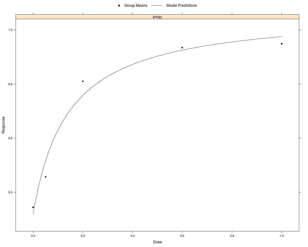
  emax 

Parameter estimates: 
emax model:
   e0  eMax  ed50 
0.322 0.746 0.142 

Dose estimate 
MED2,90% 
    0.17 
> # plots data with selected model function
> plot(dfe)
> 
> # example with IBS data
> data(IBS)
> models <- list(emax = 0.2, quadratic = -0.2, linlog = NULL)
> dfe2 <- MCPMod(IBS, models, alpha = 0.05, pVal = TRUE,
+              selModel = "aveAIC", clinRel = 0.25, off = 1)
> dfe2
MCPMod

PoC (alpha = 0.05, one-sided): yes 
Model with highest t-statistic: emax 
Models used for dose estimation: emax linlog quadratic 
Dose estimate: 
MED2,80% 
    1.57 

> # show more digits in the output
> print(dfe2, digits = 8)
MCPMod

PoC (alpha = 0.05, one-sided): yes 
Model with highest t-statistic: emax 
Models used for dose estimation: emax linlog quadratic 
Dose estimate: 
MED2,80% 
1.569525 

> summary(dfe2, digits = 8)
MCPMod

Input parameters: 
 alpha = 0.05 (one-sided) 
 model selection: aveAIC 
 prior model weights:
      emax    linlog quadratic 
0.3333333 0.3333333 0.3333333 
 clinical relevance = 0.25 
 dose estimator: MED2 (gamma = 0.1) 

Optimal Contrasts:
        emax   quadratic     linlog
0 -0.8893326 -0.81251655 -0.7437141
1  0.1348495 -0.00600689 -0.2263189
2  0.2268538  0.42048228  0.1146438
3  0.2527683  0.40366299  0.3363693
4  0.2748610 -0.00562183  0.5190199

Contrast Correlation:
               emax quadratic    linlog
emax      1.0000000 0.9200306 0.8904568
quadratic 0.9200306 1.0000000 0.7924900
linlog    0.8904568 0.7924900 1.0000000

Multiple Contrast Test:
            Tvalue     pValue
emax      3.215428 0.00182946
linlog    2.983376 0.00308837
quadratic 2.919818 0.00359480

Critical value: 1.898529

AIC criterion:
     emax    linlog quadratic 
   850.39    849.90    851.23 

Selected for dose estimation:
  emax linlog quadratic 

Model weights:
     emax    linlog quadratic 
0.3405715 0.4354486 0.2239799 

Parameter estimates: 
emax model:
       e0      eMax      ed50 
0.2171129 0.3773367 0.3628367 
linlog model:
     (Intercept) I(log(dose+off)) 
       0.2723811        0.2110124 
quadratic model:
(Intercept)        dose   I(dose^2) 
 0.24627030  0.22835783 -0.03818961 

Dose estimate 
Estimates for models
         emax linlog quadratic
MED2,80% 0.72   2.28      1.48
Model averaged dose estimate
MED2,80% 
1.569525 
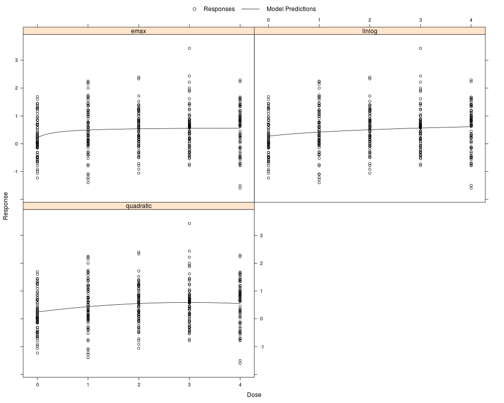
> plot(dfe2, complData = TRUE, cR = TRUE)
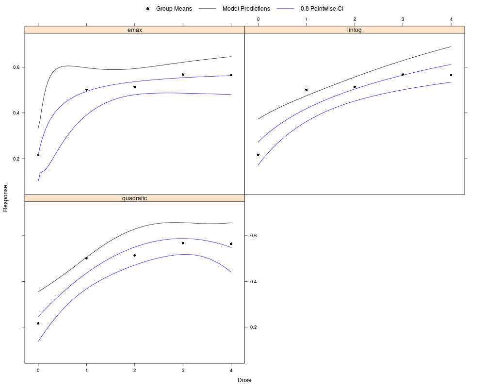
> plot(dfe2, CI = TRUE)
> 
> # simulate dose-response data
> dfData <- genDFdata(model = "emax", argsMod = c(e0 = 0.2, eMax = 1, 
+           ed50 = 0.05), doses = c(0,0.05,0.2,0.6,1), n=20, sigma=0.5)
> models <- list(emax = 0.1, logistic = c(0.2, 0.08), 
+              betaMod = c(1, 1))
> dfe3 <- MCPMod(dfData, models, clinRel = 0.4, critV = 1.891, 
+            scal = 1.5)
> 
> # (ii) Example for constructing a model list
> 
> # Contrasts to be included:
> # Model             guesstimate(s) for stand. model parameter(s) (name)
> # linear            -
> # linear in log     -
> # Emax              0.2 (ED50)
> # Emax              0.3 (ED50)
> # exponential       0.7 (delta)
> # quadratic        -0.85 (delta)
> # logistic          0.4  0.09 (ED50, delta)
> # logistic          0.3  0.1 (ED50, delta)
> # betaMod           0.3  1.3 (delta1, delta2) 
> # sigmoid Emax      0.5  2 (ED50, h)
> #
> # For each model class exactly one list entry needs to be used.
> # The names for the list entries need to be written exactly 
> # as the model functions ("linear", "linlog", "quadratic", "emax", 
> # "exponential", "logistic", "betaMod", "sigEmax").
> # For models with no parameter in the standardized model just NULL is 
> # specified as list entry.
> # For models with one parameter a vector needs to be used with length
> # equal to the number of contrasts to be used for this model class.
> # For the models with two parameters in the standardized model a vector
> # is used to hand over the contrast, if it is desired to use just one
> # contrast. Otherwise a matrix with the guesstimates in the rows needs to
> # be used. For the above example the models list has to look like this
> 
> list(linear = NULL, linlog = NULL, emax = c(0.2, 0.3),
+      exponential = 0.7, quadratic = -0.85, logistic =
+      matrix(c(0.4, 0.3, 0.09, 0.1), nrow = 2),
+      betaMod = c(0.3, 1.3), sigEmax = c(0.5, 2))
$linear
NULL

$linlog
NULL

$emax
[1] 0.2 0.3

$exponential
[1] 0.7

$quadratic
[1] -0.85

$logistic
     [,1] [,2]
[1,]  0.4 0.09
[2,]  0.3 0.10

$betaMod
[1] 0.3 1.3

$sigEmax
[1] 0.5 2.0

> 
> # Additional parameters (who will not be estimated) are the "off"
> # parameter for the linlog model and the "scal" parameter for the
> # beta model, which are not handed over in the model list.
> 
> # (iii) example for incorporation of a usermodel
> # simulate dose response data
> dats <- genDFdata("sigEmax", c(e0 = 0, eMax = 1, ed50 = 2, h = 2),
+               n = 50, sigma = 1, doses = 0:10)
> # define usermodel
> userMod <- function(dose, a, b, d){
+   a + b*dose/(dose + d)
+ }
> # define gradient
> userModGrad <- 
+     function(dose, a, b, d) cbind(1, dose/(dose+d), -b*dose/(dose+d)^2)    
> # name starting values for nls
> start <- list(userMod=c(a=0, b=1, d=2))       
> models <- list(userMod=c(0, 1, 1), linear = NULL)
> MM1 <- MCPMod(dats, models, clinRel = 0.4, selModel="AIC", start = start,
+          uGrad = userModGrad)
> 
> # (iv) Contrast matrix and critical value handed over and not calculated
> # simulate dose response data
> dat <- genDFdata(mu = (0:4)/4, n = 20, 
+                        sigma = 1, doses = (0:4)/4)
> # construct optimal contrasts and critical value with planMM
> doses <- (0:4)/4
> mods <- list(linear = NULL, quadratic = -0.7)
> pM <- planMM(mods, doses, 20)
> MCPMod(dat, models = NULL, clinRel = 0.3, contMat = pM$contMat,
+      critV = pM$critVal)
MCPMod

PoC: no 

> 
> # (v) Using MCPMod for mutiple contrast tests only
> mu1 <- c(1, 2, 2, 2, 2)                      
> mu2 <- c(1, 1, 2, 2, 2)                      
> mu3 <- c(1, 1, 1, 2, 2)                      
> mMat <- cbind(mu1, mu2, mu3)              
> dimnames(mMat)[[1]] <- doses               
> pM <- planMM(muMat = mMat, doses = doses, n = 20, cV = FALSE)
> # calculate p-values
> fit <-MCPMod(dat, models = NULL, clinRel = 0.3, contMat = pM$contMat,
+         pVal = TRUE, testOnly = TRUE)
> summary(fit)
MCPMod

Input parameters: 
 alpha = 0.025 (one-sided) 

Optimal Contrasts:
        mu1    mu2    mu3
0    -0.894 -0.548 -0.365
0.25  0.224 -0.548 -0.365
0.5   0.224  0.365 -0.365
0.75  0.224  0.365  0.548
1     0.224  0.365  0.548

Contrast Correlation:
      mu1   mu2   mu3
mu1 1.000 0.612 0.408
mu2 0.612 1.000 0.667
mu3 0.408 0.667 1.000

Multiple Contrast Test:
    Tvalue pValue
mu1  2.618  0.013
mu3  0.951  0.329
mu2  0.454  0.543

Critical value: 2.367
> 
> 
> 
> 
> 
> dev.off()
null device 
          1 
>