R Graphical Manual

Browse All

Last data update: 2014.03.03

R: Entropy plot

entropy.plot

R Documentation

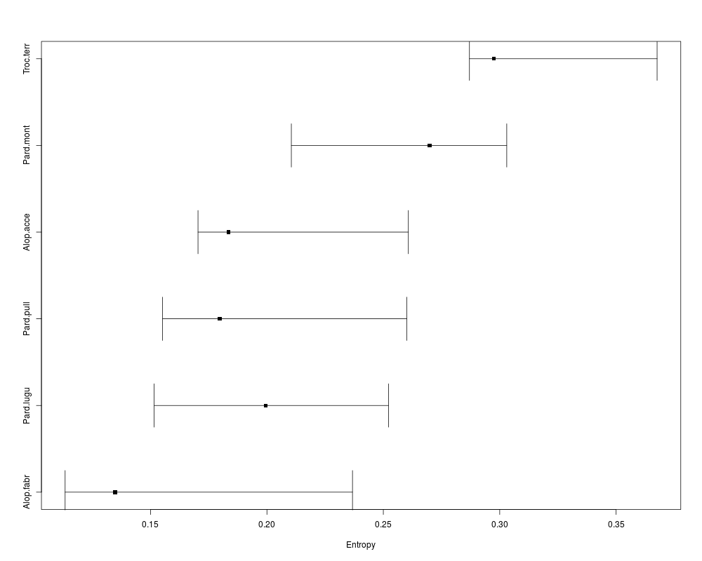
Entropy plot

Description

Plots components of entropy by species or sites.

Usage

entropy.plot(lst, y, x, ord=TRUE, type=c("species","sites")[1],
 labs, segs = TRUE, wid.seg=0.25,
 pchs = c(15,19,0,2,6,2,15,17,21,17), ...)

Arguments

`lst`	a list of `mdm` fitted models
`y`	optional – locations of the components on the vertical axis
`x`	optional – used to provide the range of the horizontal axis
`ord`	if TRUE orders the components by total entropy of each fitted model.
`type`	should the plot break down entropy by species (columns = default) or sites (rows).
`labs`	an (optional) vector of labels for species (or sites if type == "sites").
`segs`	use segments to plot end of bars as vertical lines
`wid.seg`	widths of bar ends
`pchs`	some nice plotting characters
`...`	other arguements passed to the plot function (e.g. cex).

Value

a list of plotted values of the length of lst, each component of which is of length equal to the number of species (sites).

Examples

data(spider6)
fit0 <- mdm(y2p(spider6[,1:6])~1,data=spider6)
fit1 <- mdm(y2p(spider6[,1:6])~Water+Herbs,data=spider6)
fit2 <- mdm(y2p(spider6[,1:6])~Site,data=spider6,alpha=TRUE)
anova(fit0,fit1,fit2)
entropy.plot(list(fit0,fit2,fit1))

Results


R version 3.3.1 (2016-06-21) -- "Bug in Your Hair"
Copyright (C) 2016 The R Foundation for Statistical Computing
Platform: x86_64-pc-linux-gnu (64-bit)

R is free software and comes with ABSOLUTELY NO WARRANTY.
You are welcome to redistribute it under certain conditions.
Type 'license()' or 'licence()' for distribution details.

R is a collaborative project with many contributors.
Type 'contributors()' for more information and
'citation()' on how to cite R or R packages in publications.

Type 'demo()' for some demos, 'help()' for on-line help, or
'help.start()' for an HTML browser interface to help.
Type 'q()' to quit R.

> library(MDM)
Loading required package: nnet
> png(filename="/home/ddbj/snapshot/RGM3/R_CC/result/MDM/entropy.plot.Rd_%03d_medium.png", width=480, height=480)
> ### Name: entropy.plot
> ### Title: Entropy plot
> ### Aliases: entropy.plot
> 
> ### ** Examples
> 
> data(spider6)
> fit0 <- mdm(y2p(spider6[,1:6])~1,data=spider6)
# weights:  12 (5 variable)
> fit1 <- mdm(y2p(spider6[,1:6])~Water+Herbs,data=spider6)
# weights:  24 (15 variable)
initial  value 50.169265 
iter  10 value 36.791764
iter  20 value 35.415854
iter  30 value 35.415361
final  value 35.415361 
converged
> fit2 <- mdm(y2p(spider6[,1:6])~Site,data=spider6,alpha=TRUE)
# weights:  174 (140 variable)
> anova(fit0,fit1,fit2)
Deviances, Entropies and Diversities of Parametric Diversity Models

Response: y2p(spider6[, 1:6]) 

Model 1: y2p(spider6[, 1:6]) ~ 1
Model 2: y2p(spider6[, 1:6]) ~ Water + Herbs
Model 3: y2p(spider6[, 1:6]) ~ Site 

   DF DF-Diff    Dev Dev-Diff    Ent Ent-Diff    Div Div-Ratio
1 135         94.105          1.6804          5.3680          
2 125      10 70.831  23.2748 1.2648  0.41562 3.5425    1.5153
3   0     125 60.923   9.9075 1.0879  0.17692 2.9681    1.1935
> entropy.plot(list(fit0,fit2,fit1))
> 
> 
> 
> 
> 
> dev.off()
null device 
          1 
>