R Graphical Manual

Browse All

Last data update: 2014.03.03

R: Species abundance data simulator

simdata

R Documentation

Species abundance data simulator

Description

Simulates species abundance data along a one-dimensional gradient

Usage

simdata(d, p = 10, n = 100, strip0 = TRUE, extreme = 0,
ret = TRUE, k.rand = FALSE, d.rand = TRUE, mu.rand = TRUE,
s = rep((4:8)/10, length = p), amp = c(sample(1:5), rep = TRUE,
length = p), skew = 1, ampfun, lst = FALSE, err = 1,
err.type = c("p", "n")[1], as.df = TRUE, plotit = TRUE,
ptype = "l", plty = 1, pcols = rainbow(p), add.rug = FALSE, ...)

Arguments

`d`	the (optional) locations of the species along the 1-D gradient. If d is given then it will define both the number of species and also the locations on the gradient e.g. d = rep(1:10,each=3) will generate species at locations 1,1,1,2,2,2,...,10,10,10. If d is not specified then d.rand = TRUE will randomly allocate the species modes along a gradient on [0, 1], but if d.rand = FALSE will uniformly distribute the species modes along a gradient.
`p`	number of species.
`n`	number of sites.
`strip0`	if TRUE the sites with zero total abundance are omitted.
`extreme`	number typically in the range -1 to +1 with larger numbers reducing the range of species.
`ret`	if TRUE the generated data are returned
`k.rand`	should the be random (TRUE) or fixed
`d.rand`	should the be random (TRUE) or fixed
`mu.rand`	should the be random (TRUE) or fixed
`s`	the spans of the species response curves; s is the standard deviation of the spread
`amp`	the amplitudes of the species response curves
`skew`	the skewness of the distribution; range (>0 to 5), 1 = symmetric.
`ampfun`	any function to modify the amplitude
`lst`	if lst == TRUE then both the systematic and random values are returned
`err`	if err == 0 then the values are systematic with no random variation
`err.type`	type of error; p = poison, g = gaussian
`as.df`	if return returns a data frame, otherwise a matrix
`plotit`	if TRUE then the data are plotted
`ptype`	species plot types e.g. "l" gives lines
`plty`	species plot line types
`pcols`	species plot colours
`add.rug`	should a rug be added?
`...`	other arguments passed to plot.

Value

if lst == FALSE then a data frame with variables "Locations", "Taxa.1" – "Taxa.N" where N is number of species. if lst == TRUE then two data frames "x" and "xs" with variables "Locations", "Taxa.1" – "Taxa.N" and additionally, components "sigma", "amp" and "mu" that represent the spans, amplitudes and locations of the N species along the 1-D gradient.

Examples

mydata <- simdata()
summary(mydata)
mydata <- simdata(p=5, n=50, amp=1, err=0, d.rand=FALSE,
mu.rand=FALSE, plotit = TRUE)
summary(mydata)

Results


R version 3.3.1 (2016-06-21) -- "Bug in Your Hair"
Copyright (C) 2016 The R Foundation for Statistical Computing
Platform: x86_64-pc-linux-gnu (64-bit)

R is free software and comes with ABSOLUTELY NO WARRANTY.
You are welcome to redistribute it under certain conditions.
Type 'license()' or 'licence()' for distribution details.

R is a collaborative project with many contributors.
Type 'contributors()' for more information and
'citation()' on how to cite R or R packages in publications.

Type 'demo()' for some demos, 'help()' for on-line help, or
'help.start()' for an HTML browser interface to help.
Type 'q()' to quit R.

> library(MDM)
Loading required package: nnet
> png(filename="/home/ddbj/snapshot/RGM3/R_CC/result/MDM/simdata.Rd_%03d_medium.png", width=480, height=480)
> ### Name: simdata
> ### Title: Species abundance data simulator
> ### Aliases: simdata
> 
> ### ** Examples
> 
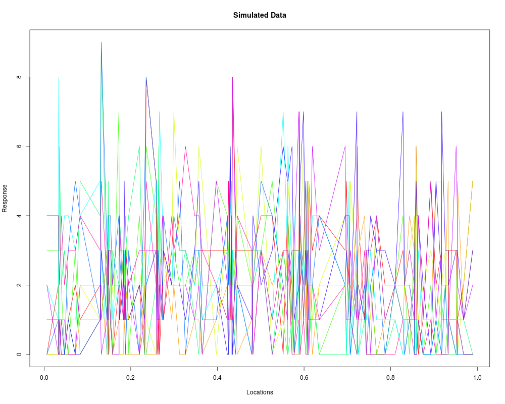
> mydata <- simdata()
> summary(mydata)
   Locations           Taxa.1        Taxa.2         Taxa.3         Taxa.4    
 Min.   :0.01293   Min.   :0.0   Min.   :0.00   Min.   :0.00   Min.   :0.00  
 1st Qu.:0.21870   1st Qu.:1.0   1st Qu.:0.00   1st Qu.:1.00   1st Qu.:1.00  
 Median :0.47162   Median :2.0   Median :1.00   Median :2.00   Median :2.00  
 Mean   :0.48870   Mean   :2.3   Mean   :1.58   Mean   :2.26   Mean   :2.13  
 3rd Qu.:0.72970   3rd Qu.:3.0   3rd Qu.:3.00   3rd Qu.:3.00   3rd Qu.:3.00  
 Max.   :0.99611   Max.   :7.0   Max.   :6.00   Max.   :6.00   Max.   :7.00  
     Taxa.5         Taxa.6         Taxa.7        Taxa.8         Taxa.9    
 Min.   :0.00   Min.   :0.00   Min.   :0.0   Min.   :0.00   Min.   :0.00  
 1st Qu.:1.00   1st Qu.:1.00   1st Qu.:1.0   1st Qu.:1.00   1st Qu.:1.00  
 Median :2.00   Median :2.00   Median :2.0   Median :2.00   Median :2.00  
 Mean   :2.49   Mean   :2.28   Mean   :2.1   Mean   :2.44   Mean   :1.99  
 3rd Qu.:3.00   3rd Qu.:3.00   3rd Qu.:3.0   3rd Qu.:3.00   3rd Qu.:3.00  
 Max.   :8.00   Max.   :9.00   Max.   :8.0   Max.   :8.00   Max.   :7.00  
    Taxa.10    
 Min.   :0.00  
 1st Qu.:1.00  
 Median :2.00  
 Mean   :2.16  
 3rd Qu.:3.00  
 Max.   :7.00  
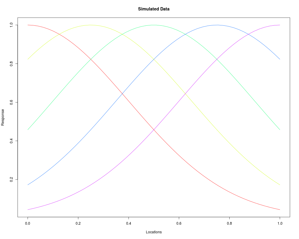
> mydata <- simdata(p=5, n=50, amp=1, err=0, d.rand=FALSE,
+ mu.rand=FALSE, plotit = TRUE)
> summary(mydata)
   Locations        Taxa.1            Taxa.2           Taxa.3      
 Min.   :0.00   Min.   :0.04394   Min.   :0.1724   Min.   :0.4578  
 1st Qu.:0.25   1st Qu.:0.17253   1st Qu.:0.4579   1st Qu.:0.6405  
 Median :0.50   Median :0.45792   Median :0.8159   Median :0.8160  
 Mean   :0.50   Mean   :0.49563   Mean   :0.7013   Mean   :0.7840  
 3rd Qu.:0.75   3rd Qu.:0.82246   3rd Qu.:0.9484   3rd Qu.:0.9465  
 Max.   :1.00   Max.   :1.00000   Max.   :0.9999   Max.   :0.9997  
     Taxa.4           Taxa.5       
 Min.   :0.1724   Min.   :0.04394  
 1st Qu.:0.4579   1st Qu.:0.17253  
 Median :0.8159   Median :0.45792  
 Mean   :0.7013   Mean   :0.49563  
 3rd Qu.:0.9484   3rd Qu.:0.82246  
 Max.   :0.9999   Max.   :1.00000  
> 
> 
> 
> 
> 
> dev.off()
null device 
          1 
>