R Graphical Manual

Browse All

Last data update: 2014.03.03

R: data.frame to array converter

df2array

R Documentation

data.frame to array converter

Description

Convert observations stored in the data.frame format into the array format.

Usage

df2array(contrast, coords, format = "any", default_value = NA, range.coords = NULL)

Arguments

`contrast`	the dataset containing the observations in rows and the contrast parameters in columns. vector or data.frame. REQUIRED.
`coords`	the spatial coordinates of the observations. matrix with a number of rows equal to the number of rows of `data`. REQUIRED.
`format`	the format of the output. Can be `"any"`,`"matrix"`,`"data.frame"` or `"list"`.
`default_value`	the element used to fill the missing observations. numeric.
`range.coords`	the maximum coordinate in each dimension to be considered. numeric vector with length equal to the number of columns of `coords`.

Details

FUNCTION:
If contrast contains several parameters, they are treated one at a time and the result is returned in the form of a list. If range.coords is NULL then the maxima coordinates are those of the coords argument. If only one parameter is specified and the format is set to "any" then a vector is returned.

Value

a list containing :

[[contrast]] : list containing the new contrast in the new format.
[[coords]] : a data.frame containing the coordinates of each observation.
[[unique_coords.group]] : two list containing the possibles coordinates in each dimension.

Examples

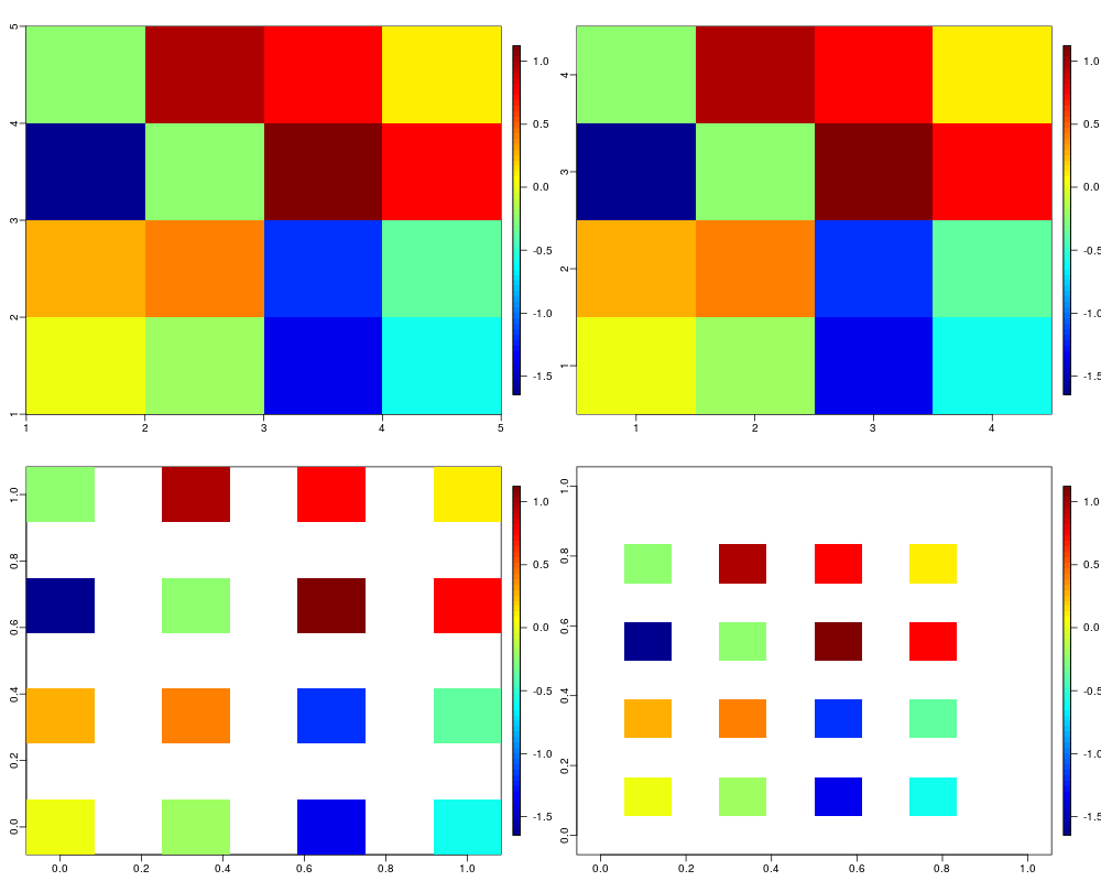
#### 1- with simulated data ####
## simulate
set.seed(10)
n <- 4
Y <- rnorm(n^2)

## conversion
res1 <- df2array(contrast = Y, coords = expand.grid(1:n + 0.5, 1:n + 0.5))
res2 <- df2array(contrast = Y, coords = expand.grid(1:n, 1:n), format = "matrix")
res3 <- df2array(contrast = Y, coords = expand.grid(2 * (1:n), 2 * (1:n)))
res4 <- df2array(contrast=cbind(Y ,Y, Y), coords = expand.grid(2 * (1:n), 2 * (1:n)),
                    range.coords = c(10,10))
					
## display
par(mfrow = c(2,2), mar = rep(2,4), mgp = c(1.5,0.5,0))
fields::image.plot(unique(res1$coords[,1]), unique(res1$coords[,2]), res1$contrast[[1]],
                   xlab = "", ylab = "")
fields::image.plot(unique(res2$coords[,1]), unique(res2$coords[,2]), res2$contrast,
                   xlab = "", ylab = "")
fields::image.plot(res3$contrast[[1]])
fields::image.plot(res4$contrast[[2]])

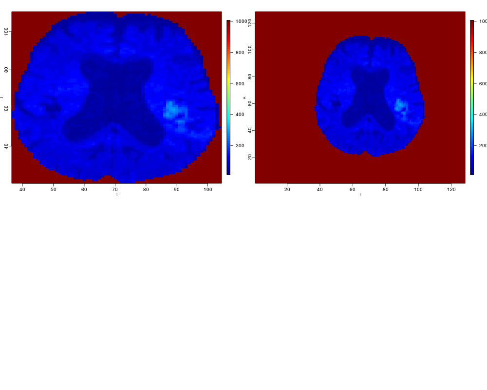
#### 2- with MRIaggr data ####
## load a MRIaggr object
data("MRIaggr.Pat1_red", package = "MRIaggr")
carto <- selectContrast(MRIaggr.Pat1_red, param = "DWI_t0", format = "vector")
coords <- selectCoords(MRIaggr.Pat1_red)
coords[,1] <- coords[,1] + 30
coords[,2] <- coords[,2] + 15

## converion 1
array.DWI_t0 <- df2array(carto, coords = coords, default_value = 1000)$contrast[[1]]

# display
fields::image.plot(min(coords[,1]):max(coords[,1]), min(coords[,2]):max(coords[,2]),
                   array.DWI_t0[,,1], xlab = "i", ylab = "j")

## conversion 2
array.DWI_t0 <- df2array(contrast=carto, coords = coords, default_value = 1000, 
                         range.coords = c(128,128,3))$contrast[[1]]

# display
fields::image.plot(1:128, 1:128, array.DWI_t0[,,1], xlab = "i", ylab = "k")

Results


R version 3.3.1 (2016-06-21) -- "Bug in Your Hair"
Copyright (C) 2016 The R Foundation for Statistical Computing
Platform: x86_64-pc-linux-gnu (64-bit)

R is free software and comes with ABSOLUTELY NO WARRANTY.
You are welcome to redistribute it under certain conditions.
Type 'license()' or 'licence()' for distribution details.

R is a collaborative project with many contributors.
Type 'contributors()' for more information and
'citation()' on how to cite R or R packages in publications.

Type 'demo()' for some demos, 'help()' for on-line help, or
'help.start()' for an HTML browser interface to help.
Type 'q()' to quit R.

> library(MRIaggr)
Loading required package: Rcpp
> png(filename="/home/ddbj/snapshot/RGM3/R_CC/result/MRIaggr/MRIaggr-df2array.Rd_%03d_medium.png", width=480, height=480)
> ### Name: df2array
> ### Title: data.frame to array converter
> ### Aliases: df2array
> ### Keywords: functions
> 
> ### ** Examples
> 
> #### 1- with simulated data ####
> ## simulate
> set.seed(10)
> n <- 4
> Y <- rnorm(n^2)
> 
> ## conversion
> res1 <- df2array(contrast = Y, coords = expand.grid(1:n + 0.5, 1:n + 0.5))
> res2 <- df2array(contrast = Y, coords = expand.grid(1:n, 1:n), format = "matrix")
> res3 <- df2array(contrast = Y, coords = expand.grid(2 * (1:n), 2 * (1:n)))
> res4 <- df2array(contrast=cbind(Y ,Y, Y), coords = expand.grid(2 * (1:n), 2 * (1:n)),
+                     range.coords = c(10,10))
> 					
> ## display
> par(mfrow = c(2,2), mar = rep(2,4), mgp = c(1.5,0.5,0))
> fields::image.plot(unique(res1$coords[,1]), unique(res1$coords[,2]), res1$contrast[[1]],
+                    xlab = "", ylab = "")
> fields::image.plot(unique(res2$coords[,1]), unique(res2$coords[,2]), res2$contrast,
+                    xlab = "", ylab = "")
> fields::image.plot(res3$contrast[[1]])
> fields::image.plot(res4$contrast[[2]])
> 
> #### 2- with MRIaggr data ####
> ## load a MRIaggr object
> data("MRIaggr.Pat1_red", package = "MRIaggr")
> carto <- selectContrast(MRIaggr.Pat1_red, param = "DWI_t0", format = "vector")
> coords <- selectCoords(MRIaggr.Pat1_red)
> coords[,1] <- coords[,1] + 30
> coords[,2] <- coords[,2] + 15
> 
> ## converion 1
> array.DWI_t0 <- df2array(carto, coords = coords, default_value = 1000)$contrast[[1]]
> 
> # display
> fields::image.plot(min(coords[,1]):max(coords[,1]), min(coords[,2]):max(coords[,2]),
+                    array.DWI_t0[,,1], xlab = "i", ylab = "j")
> 
> ## conversion 2
> array.DWI_t0 <- df2array(contrast=carto, coords = coords, default_value = 1000, 
+                          range.coords = c(128,128,3))$contrast[[1]]
> 
> # display
> fields::image.plot(1:128, 1:128, array.DWI_t0[,,1], xlab = "i", ylab = "k")
> 
> 
> 
> 
> 
> 
> dev.off()
null device 
          1 
>