Last data update: 2014.03.03
R: Spatial regularization using ICM
Spatial regularization using ICM
Description
Interface to C++ functions that perform spatial regularization of probabilistic group membership using Iterated Conditional Means.
Usage
calcPotts(W_SR, sample, rho, prior = TRUE, site_order = NULL, W_LR = NULL,
         nbGroup_min = 100, coords = NULL, distance.ref = NULL, threshold = 0.1,
		 multiV = TRUE, iter_max = 200, cv.criterion = 0.005, verbose = 2)
Arguments
W_SR
The local neighborhood matrix. dgCMatrix . Should be normalized by row (i.e. rowSums(W_SR)=1). REQUIRED.
sample
The initial group probability membership. numeric vector . REQUIRED.
rho
Value of the spatial regularisation parameters. numeric vector . REQUIRED.
prior
Should the sample values be used as a prior ? logical .
site_order
a specific order to go all over the sites. integer vector .
W_LR
The regional neighborhood matrix. dgCMatrix . Should contain the distances between the observations (0 indicating infinite distance).
nbGroup_min
The minimum group size of the spatial groups required for performing regional regularization. integer .
coords
The voxel coordinates. matrix .
distance.ref
The intervals of distance defining the several neighborhood orders in W_LR. numeric vector .
threshold
The minimum value to consider non-negligible group membership. numeric .
multiV
Should the regional potential range be specific to each spatial group ? logical .
iter_max
Maximum number of ICM iterations. integer .
cv.criterion
Convergence criterion of the ICM . numeric .
verbose
should the ICM be be traced over iterations ? logical . 1 to display each iteration and 2 to display convergence diagnostics.
Details
The convergence criterion of the ICM is computed as maximum absolute difference between the group membership probability between two consecutive iterations.
Examples
optionsMRIaggr(legend=FALSE,axes=FALSE,num.main=FALSE,mar=c(0,2,2,0))
# spatial field
## Not run:
n <- 30
## End(Not run)
G <- 3
coords <- which(matrix(0, nrow = n * G, ncol = n * G) == 0,arr.ind = TRUE)
# neighborhood matrix
W_SR <- calcW(as.data.frame(coords), range = sqrt(2), row.norm = TRUE)$W
resW <- calcW(as.data.frame(coords), range = 10, row.norm = FALSE, calcBlockW = TRUE)
W_LR <- resW$W
site_order <- unlist(resW$blocks$ls_groups) - 1
# initialisation
set.seed(10)
system.time(
sample <- simulPotts(W_SR, G = 3, rho = 3.5, iter_max = 500,
site_order = site_order)$simulation
)
intensity <- rnorm((n * G)^2, mean = apply(sample, 1, which.max), sd = 0.5)
likelihood <- matrix(unlist(lapply(1:3, function(x){dnorm(intensity, mean = x, sd = 0.5)})),
ncol = G, nrow = (n * G)^2, byrow = FALSE)
likelihood_sqrt <- sqrt(likelihood)
probability <- sweep(likelihood_sqrt, MARGIN = 1, FUN = "/", STATS = rowSums(likelihood_sqrt))
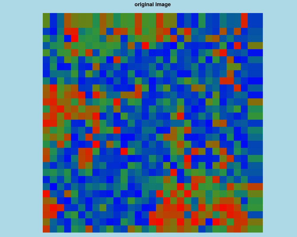
multiplot(as.data.frame(coords), probability, palette = "rgb",
main = "original image")
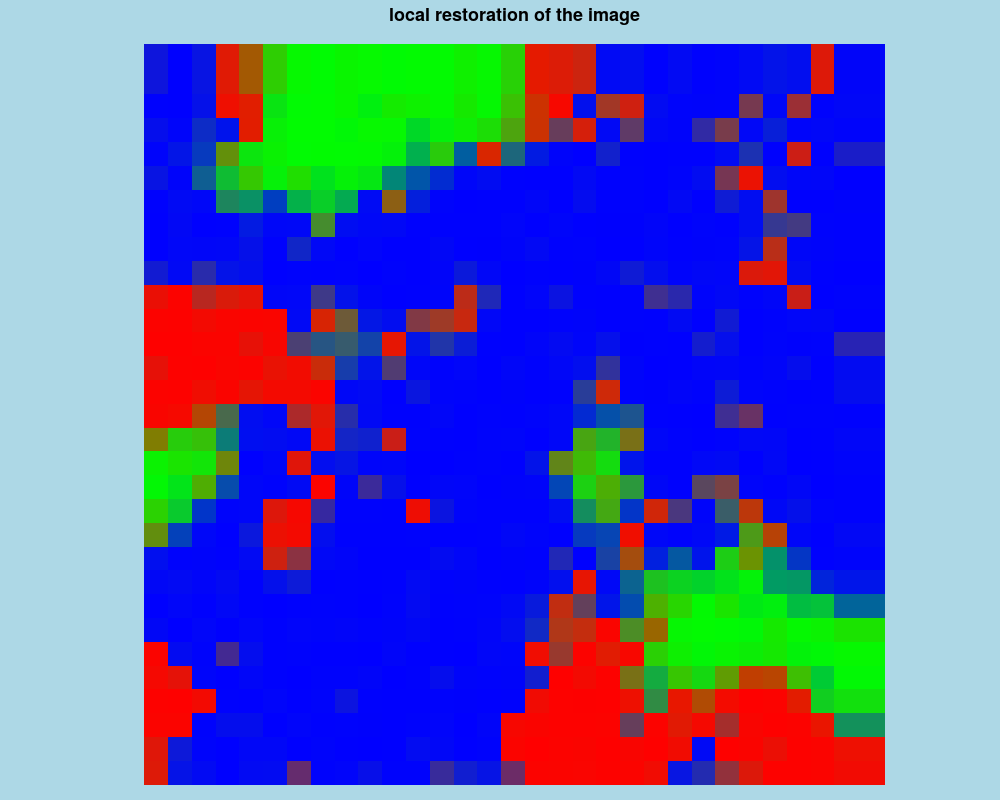
#### local image restoration
LocalRestoration <- calcPotts(W_SR = W_SR, sample = probability, rho = 4,
site_order = site_order)
multiplot(as.data.frame(coords), LocalRestoration$predicted, palette = "rgb",
main = "local restoration of the image")
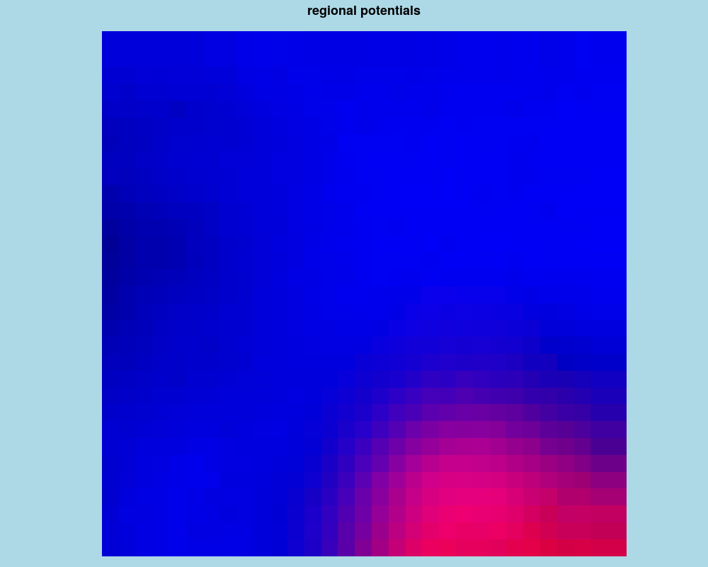
#### regional image restoration
distance.ref <- seq(1, 10, 1)
RegionalRestoration <- calcPotts(W_SR = W_SR, sample = probability,
rho = c(4,2), site_order = site_order,
W_LR = W_LR, coords = coords, distance.ref = distance.ref)
# regional potential
multiplot(as.data.frame(coords),
matrix(unlist(RegionalRestoration$Vregional), ncol = 3, nrow = (n * G)^2, byrow = FALSE),
palette = "rgb", main = "regional potentials")
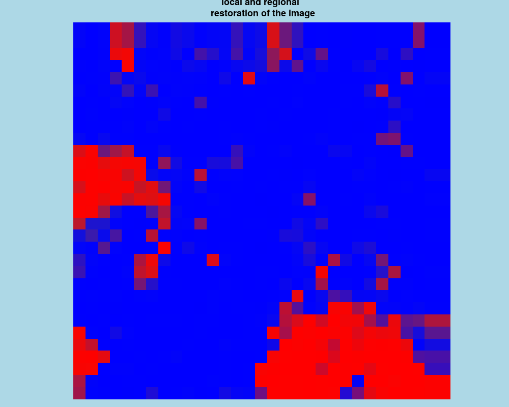
# final image
multiplot(as.data.frame(coords),
matrix(unlist(RegionalRestoration$predicted), ncol = 3, nrow = (n * G)^2, byrow = FALSE),
palette = "rgb", main = "local and regional \n restoration of the image")
Results
R version 3.3.1 (2016-06-21) -- "Bug in Your Hair"
Copyright (C) 2016 The R Foundation for Statistical Computing
Platform: x86_64-pc-linux-gnu (64-bit)

R is free software and comes with ABSOLUTELY NO WARRANTY.
You are welcome to redistribute it under certain conditions.
Type 'license()' or 'licence()' for distribution details.

R is a collaborative project with many contributors.
Type 'contributors()' for more information and
'citation()' on how to cite R or R packages in publications.

Type 'demo()' for some demos, 'help()' for on-line help, or
'help.start()' for an HTML browser interface to help.
Type 'q()' to quit R.

> library(MRIaggr)
Loading required package: Rcpp
> png(filename="/home/ddbj/snapshot/RGM3/R_CC/result/MRIaggr/sfMM-calcPotts.Rd_%03d_medium.png", width=480, height=480)
> ### Name: calcPotts
> ### Title: Spatial regularization using ICM
> ### Aliases: calcPotts
>
> ### ** Examples
>
> optionsMRIaggr(legend=FALSE,axes=FALSE,num.main=FALSE,mar=c(0,2,2,0))
>
> # spatial field
> ## Not run:
> ##D n <- 30
> ## End(Not run)
> ## Don't show:
> n <- 10
> ## End(Don't show)
> G <- 3
> coords <- which(matrix(0, nrow = n * G, ncol = n * G) == 0,arr.ind = TRUE)
>
> # neighborhood matrix
> W_SR <- calcW(as.data.frame(coords), range = sqrt(2), row.norm = TRUE)$W
> resW <- calcW(as.data.frame(coords), range = 10, row.norm = FALSE, calcBlockW = TRUE)
> W_LR <- resW$W
> site_order <- unlist(resW$blocks$ls_groups) - 1
>
> # initialisation
> set.seed(10)
> system.time(
+ sample <- simulPotts(W_SR, G = 3, rho = 3.5, iter_max = 500,
+      site_order = site_order)$simulation
+ )
0% 10   20   30   40   50   60   70   80   90   100%
|----|----|----|----|----|----|----|----|----|----|
**************************************************|
|
   user  system elapsed
  0.100   0.000   0.099
>
> intensity <- rnorm((n * G)^2, mean = apply(sample, 1, which.max), sd = 0.5)
> likelihood <- matrix(unlist(lapply(1:3, function(x){dnorm(intensity, mean = x, sd = 0.5)})),
+      ncol = G, nrow = (n * G)^2, byrow = FALSE)
> likelihood_sqrt <- sqrt(likelihood)
>
> probability <- sweep(likelihood_sqrt, MARGIN = 1, FUN = "/", STATS = rowSums(likelihood_sqrt))
>
> multiplot(as.data.frame(coords), probability, palette = "rgb",
+      main = "original image")
>
> #### local image restoration
> LocalRestoration <- calcPotts(W_SR = W_SR, sample = probability, rho = 4,
+      site_order = site_order)
iteration 1 : totaldiff = 377.477 | maxdiff = 0.719846
iteration 2 : totaldiff = 126.706 | maxdiff = 0.461399
iteration 3 : totaldiff = 37.6441 | maxdiff = 0.197652
iteration 4 : totaldiff = 15.3192 | maxdiff = 0.131896
iteration 5 : totaldiff = 7.86262 | maxdiff = 0.0863482
iteration 6 : totaldiff = 4.561 | maxdiff = 0.0553534
iteration 7 : totaldiff = 2.86262 | maxdiff = 0.0393689
iteration 8 : totaldiff = 1.89935 | maxdiff = 0.0271843
iteration 9 : totaldiff = 1.31207 | maxdiff = 0.0230567
iteration 10 : totaldiff = 0.938505 | maxdiff = 0.0207437
iteration 11 : totaldiff = 0.694233 | maxdiff = 0.0186982
iteration 12 : totaldiff = 0.531938 | maxdiff = 0.0168628
iteration 13 : totaldiff = 0.42073 | maxdiff = 0.0151973
iteration 14 : totaldiff = 0.34252 | maxdiff = 0.013675
iteration 15 : totaldiff = 0.285769 | maxdiff = 0.0122937
iteration 16 : totaldiff = 0.242721 | maxdiff = 0.0110251
iteration 17 : totaldiff = 0.208744 | maxdiff = 0.00985519
iteration 18 : totaldiff = 0.181017 | maxdiff = 0.00878157
iteration 19 : totaldiff = 0.157821 | maxdiff = 0.0078014
iteration 20 : totaldiff = 0.138047 | maxdiff = 0.0069112
iteration 21 : totaldiff = 0.120965 | maxdiff = 0.00610681
iteration 22 : totaldiff = 0.106074 | maxdiff = 0.00538341
iteration 23 : totaldiff = 0.0930191 | maxdiff = 0.00473571
>
> multiplot(as.data.frame(coords), LocalRestoration$predicted, palette = "rgb",
+      main = "local restoration of the image")
>
> #### regional image restoration
> distance.ref <- seq(1, 10, 1)
>
> RegionalRestoration <- calcPotts(W_SR = W_SR, sample = probability,
+      rho = c(4,2), site_order = site_order,
+      W_LR = W_LR, coords = coords, distance.ref = distance.ref)
iteration 1 : totaldiff = 451.389 | maxdiff = 0.784689
iteration 2 : totaldiff = 157.917 | maxdiff = 0.583253
iteration 3 : totaldiff = 94.7593 | maxdiff = 0.510262
iteration 4 : totaldiff = 60.7116 | maxdiff = 0.415989
iteration 5 : totaldiff = 40.2135 | maxdiff = 0.493415
iteration 6 : totaldiff = 25.5837 | maxdiff = 0.315286
iteration 7 : totaldiff = 17.2948 | maxdiff = 0.387792
iteration 8 : totaldiff = 14.0267 | maxdiff = 0.342669
iteration 9 : totaldiff = 12.6206 | maxdiff = 0.523771
iteration 10 : totaldiff = 9.70745 | maxdiff = 0.417766
iteration 11 : totaldiff = 7.00181 | maxdiff = 0.305046
iteration 12 : totaldiff = 5.73897 | maxdiff = 0.278059
iteration 13 : totaldiff = 4.08077 | maxdiff = 0.223751
iteration 14 : totaldiff = 2.07393 | maxdiff = 0.140449
iteration 15 : totaldiff = 0.969519 | maxdiff = 0.0604498
iteration 16 : totaldiff = 0.451038 | maxdiff = 0.0236845
iteration 17 : totaldiff = 0.224973 | maxdiff = 0.0136769
iteration 18 : totaldiff = 0.122385 | maxdiff = 0.00774178
iteration 19 : totaldiff = 0.0709919 | maxdiff = 0.00438846
iteration 20 : totaldiff = 0.919245 | maxdiff = 0.0283198
iteration 21 : totaldiff = 0.403364 | maxdiff = 0.0189132
iteration 22 : totaldiff = 0.218222 | maxdiff = 0.0125333
iteration 23 : totaldiff = 0.130883 | maxdiff = 0.00782152
iteration 24 : totaldiff = 0.0828992 | maxdiff = 0.00486518
iteration 25 : totaldiff = 0.275483 | maxdiff = 0.00790047
iteration 26 : totaldiff = 0.14834 | maxdiff = 0.00521008
iteration 27 : totaldiff = 0.0913053 | maxdiff = 0.0040836
iteration 28 : totaldiff = 0.14551 | maxdiff = 0.00602982
iteration 29 : totaldiff = 0.0893481 | maxdiff = 0.00455238
iteration 30 : totaldiff = 0.104816 | maxdiff = 0.00547746
iteration 31 : totaldiff = 0.0666083 | maxdiff = 0.00401763
iteration 32 : totaldiff = 0.0808827 | maxdiff = 0.00470659
 Group  1  - radius :  4.15
 Group  2  - radius :
 Group  3  - radius :  10.92
>
> # regional potential
> multiplot(as.data.frame(coords),
+      matrix(unlist(RegionalRestoration$Vregional), ncol = 3, nrow = (n * G)^2, byrow = FALSE),
+      palette = "rgb", main = "regional potentials")
>
> # final image
> multiplot(as.data.frame(coords),
+      matrix(unlist(RegionalRestoration$predicted), ncol = 3, nrow = (n * G)^2, byrow = FALSE),
+      palette = "rgb", main = "local and regional \n restoration of the image")
>
>
>
>
>
> dev.off()
null device
          1
>
 .
.