a matrix containing the observations (by rows) for the various groups (by columns). REQUIRED.
W_SR
the local neighbourhood matrix. dgCMatrix. Should be normalized by row (i.e. rowSums(Wweight_SR)=1). REQUIRED.
rho_max
Maximum possible rho value (numeric), minimum is 0.
prior_prevalence
should a prior on class prevalence be including when estimating the regularisation parameters ? logical.
test.regional
Should regional regularization be considered. logical.
W_LR
the regional neighbourhood matrix. dgCMatrix. Should be contains the distances between the observations (0 indicating infinite distance).
distance.ref
the interval of distance defining the several neighbourhood orders in W_LR. numeric vector.
threshold
the minimum value of the posterior probability for group G for being considered as lesioned when forming the spatial groups. double.
nbGroup_min
the minimum group size of the spatial groups required for computing the regional potential. integer.
coords
coordinates of each site. matrix.
regionalGroups
how should the regional potential be computed : last group versus the others ("last_vs_others") or for each group ("each").
multiV
should the regional neighbourhood range be computed for each spatial group ? logical.
Value
A numericVector containing the estimated regularisation parameter(s).
See Also
calcW to compute the neighbourhood matrix, simulPotts to draw simulations from a Potts model. rhoLvfree to estimate the regularization parameters using mean field approximation.
calcPottsParameter general interface for estimating the regularization parameters.
Examples
# spatial field
## Not run:
n <- 50
## End(Not run)
G <- 3
coords <- which(matrix(0, nrow = n * G, ncol = n * G) == 0,arr.ind = TRUE)
# neighbourhood matrix
W_SR <- calcW(as.data.frame(coords), range = sqrt(2), row.norm = TRUE)$W
W_LR <- calcW(as.data.frame(coords), range = 10, row.norm = FALSE)$W
# initialisation
set.seed(10)
sample <- simulPotts(W_SR, G = 3, rho = 3.5, iter_max = 500,
site_order = TRUE)$simulation
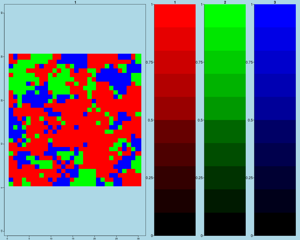
multiplot(as.data.frame(coords), sample,palette = "rgb")
# estimation
rho <- rhoMF(Y=sample, W_SR = W_SR)
rho
# the regional potential is computed for each group
rho <- rhoMF(Y = sample, W_SR = W_SR,
test.regional = TRUE, W_LR = W_LR, distance.ref = seq(1, 10, 0.5),
coords = coords, regionalGroups = "each")
rho
# the regional potential is computed for the last group vs. the others
rho <- rhoMF(Y = sample, W_SR = W_SR,
test.regional = TRUE, W_LR = W_LR, distance.ref = seq(1, 10, 0.5),
coords = coords, regionalGroups = "last_vs_others")
rho
Results
R version 3.3.1 (2016-06-21) -- "Bug in Your Hair"
Copyright (C) 2016 The R Foundation for Statistical Computing
Platform: x86_64-pc-linux-gnu (64-bit)

R is free software and comes with ABSOLUTELY NO WARRANTY.
You are welcome to redistribute it under certain conditions.
Type 'license()' or 'licence()' for distribution details.

R is a collaborative project with many contributors.
Type 'contributors()' for more information and
'citation()' on how to cite R or R packages in publications.

Type 'demo()' for some demos, 'help()' for on-line help, or
'help.start()' for an HTML browser interface to help.
Type 'q()' to quit R.

> library(MRIaggr)
Loading required package: Rcpp
> png(filename="/home/ddbj/snapshot/RGM3/R_CC/result/MRIaggr/sfMM-rhoMF.Rd_%03d_medium.png", width=480, height=480)
> ### Name: rhoMF
> ### Title: Estimation of the local and regional spatial correlation
> ### Aliases: rhoMF
>
> ### ** Examples
>
> # spatial field
> ## Not run:
> ##D n <- 50
> ## End(Not run)
> ## Don't show:
> n <- 10
> ## End(Don't show)
> G <- 3
> coords <- which(matrix(0, nrow = n * G, ncol = n * G) == 0,arr.ind = TRUE)
>
> # neighbourhood matrix
> W_SR <- calcW(as.data.frame(coords), range = sqrt(2), row.norm = TRUE)$W
> W_LR <- calcW(as.data.frame(coords), range = 10, row.norm = FALSE)$W
>
> # initialisation
> set.seed(10)
> sample <- simulPotts(W_SR, G = 3, rho = 3.5, iter_max = 500,
+                      site_order = TRUE)$simulation
0% 10   20   30   40   50   60   70   80   90   100%
|----|----|----|----|----|----|----|----|----|----|
**************************************************|
|
0% 10   20   30   40   50   60   70   80   90   100%
|----|----|----|----|----|----|----|----|----|----|
**************************************************|
|
>
> multiplot(as.data.frame(coords), sample,palette = "rgb")
>
> # estimation
> rho <- rhoMF(Y=sample, W_SR = W_SR)
> rho
[1] 3.684189
>
> # the regional potential is computed for each group
> rho <- rhoMF(Y = sample, W_SR = W_SR,
+              test.regional = TRUE, W_LR = W_LR, distance.ref = seq(1, 10, 0.5),
+ 			 coords = coords, regionalGroups = "each")
> rho
[1] 1.207717 6.258988
>
> # the regional potential is computed for the last group vs. the others
> rho <- rhoMF(Y = sample, W_SR = W_SR,
+              test.regional = TRUE, W_LR = W_LR, distance.ref = seq(1, 10, 0.5),
+ 			 coords = coords, regionalGroups = "last_vs_others")
> rho
[1]  3.190126 16.414513
>
>
>
>
>
> dev.off()
null device
          1
>
 .
.