Visualization for sample size calculation

Description

To illustrate the relationship of desired fold change and the calculated minimal number sample size which are (1) number of biological replicates per condition, (2) number of peptides per protein, (3) number of transitions per peptide, and (4) power. The input is the result from function (designSampleSize.

Usage

designSampleSizePlots(data=data)

Arguments

Details

Data in the example is based on the results of sample size calculation from function designSampleSize.

Author(s)

Ching-Yun Chang, Meena Choi, Olga Vitek.

Maintainer: Meena Choi (mnchoi67@gmail.com)

References

Meena Choi, Ching-Yun Chang, Timothy Clough, Daniel Broudy, Trevor Killeen, Brendan MacLean and Olga Vitek. "MSstats: an R package for statistical analysis of quantitative mass spectrometry-based proteomic experiments" Bioinformatics, 30(17):2524-2526, 2014.

Ching-Yun Chang, Paola Picotti, Ruth Huttenhain, Viola Heinzelmann-Schwarz, Marko Jovanovic, Ruedi Aebersold, Olga Vitek. "Protein significance analysis in selected reaction monitoring (SRM) measurements." Molecular & Cellular Proteomics, 11:M111.014662, 2012.

Timothy Clough, Safia Thaminy, Susanne Ragg, Ruedi Aebersold, Olga Vitek. "Statistical protein quantification and significance analysis in label-free LC-M experiments with complex designs" BMC Bioinformatics, 13:S16, 2012.

Examples

# Based on the results of sample size calculation from function designSampleSize, we generate a series of sample size plots for number of biological replicates, or peptides, or transitions or power plot.

QuantData<-dataProcess(SRMRawData)
head(QuantData$ProcessedData)

## based on multiple comparisons  (T1 vs T3; T1 vs T7; T1 vs T9)
comparison1<-matrix(c(-1,0,1,0,0,0,0,0,0,0),nrow=1)
comparison2<-matrix(c(-1,0,0,0,0,0,1,0,0,0),nrow=1)
comparison3<-matrix(c(-1,0,0,0,0,0,0,0,1,0),nrow=1)
comparison<-rbind(comparison1,comparison2, comparison3)
row.names(comparison)<-c("T3-T1","T7-T1","T9-T1")

testResultMultiComparisons<-groupComparison(contrast.matrix=comparison,data=QuantData)


## plot the calculated sample sizes for future experiments:

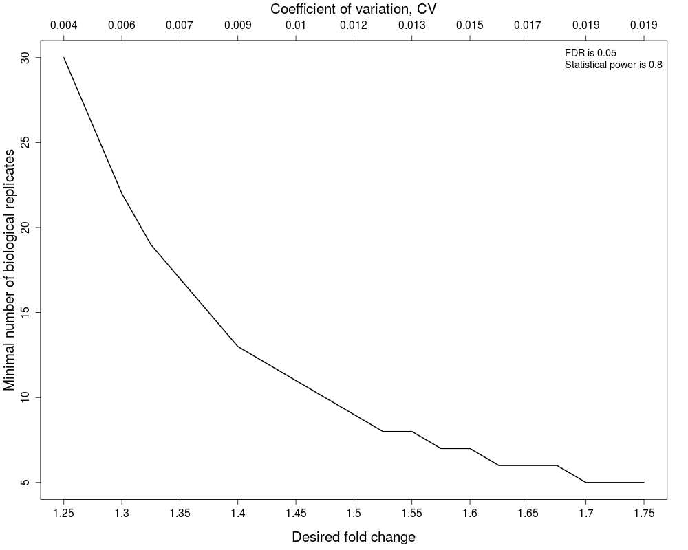
#(1) Minimal number of biological replicates per condition

result.sample<-designSampleSize(data=testResultMultiComparisons$fittedmodel,numSample=TRUE,desiredFC=c(1.25,1.75),FDR=0.05,power=0.8)
designSampleSizePlots(data=result.sample)

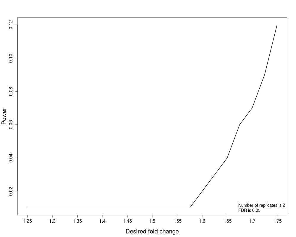
#(2) Power

result.power<-designSampleSize(data=testResultMultiComparisons$fittedmodel,numSample=2,desiredFC=c(1.25,1.75),FDR=0.05,power=TRUE)
designSampleSizePlots(data=result.power)

Results

R version 3.3.1 (2016-06-21) -- "Bug in Your Hair"
Copyright (C) 2016 The R Foundation for Statistical Computing
Platform: x86_64-pc-linux-gnu (64-bit)

R is free software and comes with ABSOLUTELY NO WARRANTY.
You are welcome to redistribute it under certain conditions.
Type 'license()' or 'licence()' for distribution details.

R is a collaborative project with many contributors.
Type 'contributors()' for more information and
'citation()' on how to cite R or R packages in publications.

Type 'demo()' for some demos, 'help()' for on-line help, or
'help.start()' for an HTML browser interface to help.
Type 'q()' to quit R.

> library(MSstats)
Loading required package: ggplot2
Loading required package: Rcpp
Loading required package: grid
Loading required package: reshape2
Warning message:
replacing previous import 'reshape::melt' by 'data.table::melt' when loading 'MSstats' 
> png(filename="/home/ddbj/snapshot/RGM3/R_BC/result/MSstats/designSampleSizePlots.Rd_%03d_medium.png", width=480, height=480)
> ### Name: designSampleSizePlots
> ### Title: Visualization for sample size calculation
> ### Aliases: designSampleSizePlots
> 
> ### ** Examples
> 
> # Based on the results of sample size calculation from function designSampleSize, we generate a series of sample size plots for number of biological replicates, or peptides, or transitions or power plot.
> 
> QuantData<-dataProcess(SRMRawData)

 DONE : Incomplete rows for missing peaks are added with intensity values=NA. 

* Use all features that the dataset origianally has.
                       
  Summary of Features :
                         count
# of Protein                 2
# of Peptides/Protein      2-2
# of Transitions/Peptide   3-3
                      
  Summary of Samples :
                           1 2 3 4 5 6 7 8 9 10
# of MS runs               3 3 3 3 3 3 3 3 3  3
# of Biological Replicates 3 3 3 3 3 3 3 3 3  3
# of Technical Replicates  1 1 1 1 1 1 1 1 1  1

 Summary of Missingness :

  # transitions are completely missing in one condition: 0


  # run with 75% missing observations: 0


 == Start the summarization per subplot...
Getting the summarization by Tukey's median polish per subplot for protein  IDHC ( 1  of  2 )
Getting the summarization by Tukey's median polish per subplot for protein  PMG2 ( 2  of  2 )

 == the summarization per subplot is done.
> head(QuantData$ProcessedData)
   PROTEIN             PEPTIDE TRANSITION                    FEATURE LABEL
1     IDHC     ATDVIVPEEGELR_2      y7_NA      ATDVIVPEEGELR_2_y7_NA     H
3     IDHC     ATDVIVPEEGELR_2      y8_NA      ATDVIVPEEGELR_2_y8_NA     H
5     IDHC     ATDVIVPEEGELR_2      y9_NA      ATDVIVPEEGELR_2_y9_NA     H
7     IDHC DQTNDQVTVDSATATLK_2     y10_NA DQTNDQVTVDSATATLK_2_y10_NA     H
9     IDHC DQTNDQVTVDSATATLK_2     y11_NA DQTNDQVTVDSATATLK_2_y11_NA     H
11    IDHC DQTNDQVTVDSATATLK_2      y8_NA  DQTNDQVTVDSATATLK_2_y8_NA     H
   GROUP_ORIGINAL SUBJECT_ORIGINAL RUN GROUP SUBJECT SUBJECT_NESTED INTENSITY
1               1            ReplA   1     0       0            0.0 84361.083
3               1            ReplA   1     0       0            0.0 29778.102
5               1            ReplA   1     0       0            0.0 17921.293
7               1            ReplA   1     0       0            0.0  4481.229
9               1            ReplA   1     0       0            0.0  1871.042
11              1            ReplA   1     0       0            0.0  2640.060
   ABUNDANCE METHOD SuggestToFilter
1   15.85586      1               0
3   14.35353      1               0
5   13.62096      1               0
7   11.62125      1               0
9   10.36120      1               0
11  10.85792      1               0
> 
> ## based on multiple comparisons  (T1 vs T3; T1 vs T7; T1 vs T9)
> comparison1<-matrix(c(-1,0,1,0,0,0,0,0,0,0),nrow=1)
> comparison2<-matrix(c(-1,0,0,0,0,0,1,0,0,0),nrow=1)
> comparison3<-matrix(c(-1,0,0,0,0,0,0,0,1,0),nrow=1)
> comparison<-rbind(comparison1,comparison2, comparison3)
> row.names(comparison)<-c("T3-T1","T7-T1","T9-T1")
> 
> testResultMultiComparisons<-groupComparison(contrast.matrix=comparison,data=QuantData)

 Start to test and get inference in whole plot...
Testing a comparison for protein  IDHC ( 1  of  2 )
Testing a comparison for protein  PMG2 ( 2  of  2 )
Warning messages:
1: In if (is.na(tempresult$result$pvalue)) { :
  the condition has length > 1 and only the first element will be used
2: In if (is.na(tempresult$result$pvalue)) { :
  the condition has length > 1 and only the first element will be used
> 
> 
> ## plot the calculated sample sizes for future experiments:
> 
> #(1) Minimal number of biological replicates per condition
> 
> result.sample<-designSampleSize(data=testResultMultiComparisons$fittedmodel,numSample=TRUE,desiredFC=c(1.25,1.75),FDR=0.05,power=0.8)
> designSampleSizePlots(data=result.sample)
> 
> #(2) Power
> 
> result.power<-designSampleSize(data=testResultMultiComparisons$fittedmodel,numSample=2,desiredFC=c(1.25,1.75),FDR=0.05,power=TRUE)
> designSampleSizePlots(data=result.power)
> 
> 
> 
> 
> 
> 
> 
> dev.off()
null device 
          1 
>