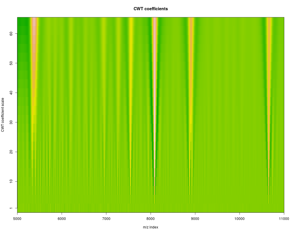
Continuous Wavelet Transform (CWT)

Description

CWT(Continuous Wavelet Transform) with Mexican Hat wavelet (by default) to match the peaks in Mass Spectrometry spectrum

Usage

cwt(ms, scales = 1, wavelet = "mexh")

Arguments

Value

The return is the 2-D CWT coefficient matrix, with column names as the scale. Each column is the CWT coefficients at that scale.

Author(s)

Pan Du, Simon Lin

Examples

	data(exampleMS)
	scales <- seq(1, 64, 3)
	wCoefs <- cwt(exampleMS[5000:11000], scales=scales, wavelet='mexh')

	## Plot the 2-D CWT coefficients as image (It may take a while!)
	xTickInterval <- 1000
	image(5000:11000, scales, wCoefs, col=terrain.colors(256), axes=FALSE, xlab='m/z index', ylab='CWT coefficient scale', main='CWT coefficients')
	axis(1, at=seq(5000, 11000, by=xTickInterval))
	axis(2, at=c(1, seq(10, 64, by=10)))
	box()

Results

R version 3.3.1 (2016-06-21) -- "Bug in Your Hair"
Copyright (C) 2016 The R Foundation for Statistical Computing
Platform: x86_64-pc-linux-gnu (64-bit)

R is free software and comes with ABSOLUTELY NO WARRANTY.
You are welcome to redistribute it under certain conditions.
Type 'license()' or 'licence()' for distribution details.

R is a collaborative project with many contributors.
Type 'contributors()' for more information and
'citation()' on how to cite R or R packages in publications.

Type 'demo()' for some demos, 'help()' for on-line help, or
'help.start()' for an HTML browser interface to help.
Type 'q()' to quit R.

> library(MassSpecWavelet)
Loading required package: waveslim

waveslim: Wavelet Method for 1/2/3D Signals (version = 1.7.5)

> png(filename="/home/ddbj/snapshot/RGM3/R_BC/result/MassSpecWavelet/cwt.Rd_%03d_medium.png", width=480, height=480)
> ### Name: cwt
> ### Title: Continuous Wavelet Transform (CWT)
> ### Aliases: cwt
> ### Keywords: methods
> 
> ### ** Examples
> 
> 	data(exampleMS)
> 	scales <- seq(1, 64, 3)
> 	wCoefs <- cwt(exampleMS[5000:11000], scales=scales, wavelet='mexh')
> 
> 	## Plot the 2-D CWT coefficients as image (It may take a while!)
> 	xTickInterval <- 1000
> 	image(5000:11000, scales, wCoefs, col=terrain.colors(256), axes=FALSE, xlab='m/z index', ylab='CWT coefficient scale', main='CWT coefficients')
> 	axis(1, at=seq(5000, 11000, by=xTickInterval))
> 	axis(2, at=c(1, seq(10, 64, by=10)))
> 	box()
> 
> 
> 
> 
> 
> dev.off()
null device 
          1 
>