Supported by Dr. Osamu Ogasawara and  . . |
|
Last data update: 2014.03.03 |
Methods for image() in Package 'Matrix'DescriptionMethods for function The Matrix package Usage
## S4 method for signature 'dgTMatrix'
image(x,
xlim = c(1, di[2]),
ylim = c(di[1], 1), aspect = "iso",
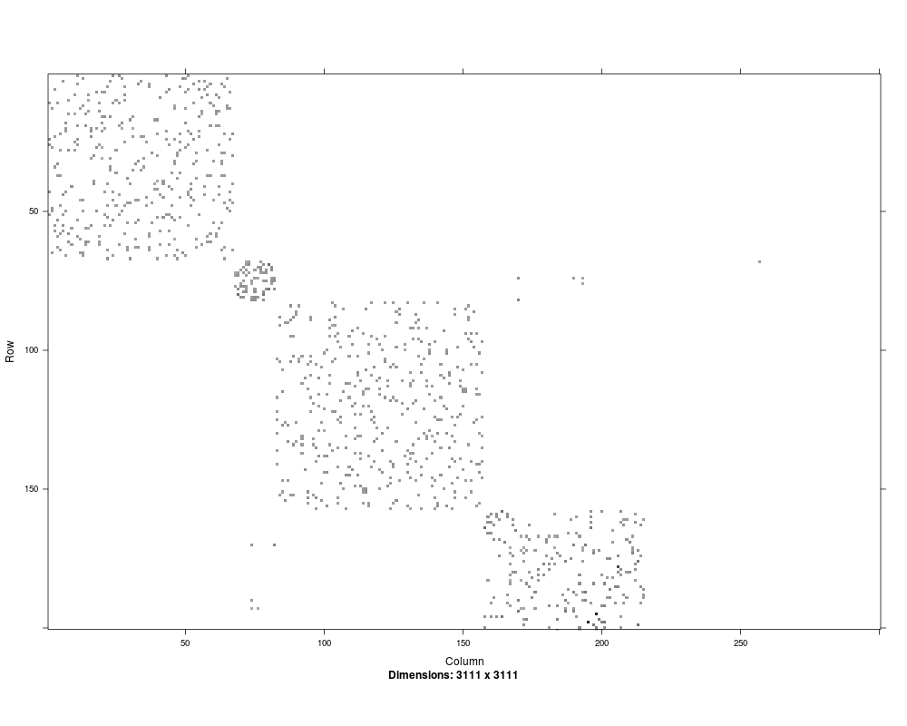
sub = sprintf("Dimensions: %d x %d", di[1], di[2]),
xlab = "Column", ylab = "Row", cuts = 15,
useRaster = FALSE,
useAbs = NULL, colorkey = !useAbs,
col.regions = NULL,
lwd = NULL, ...)
Arguments
Valueas all lattice graphics functions, MethodsAll methods currently end up calling the method for the
See Also
Examples
showMethods(image)
## If you want to see all the methods' implementations:
showMethods(image, incl=TRUE, inherit=FALSE)
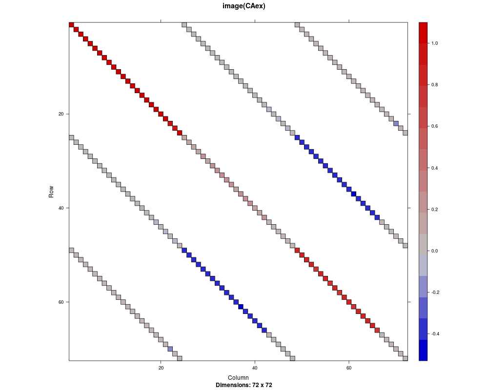
data(CAex)
image(CAex, main = "image(CAex)")
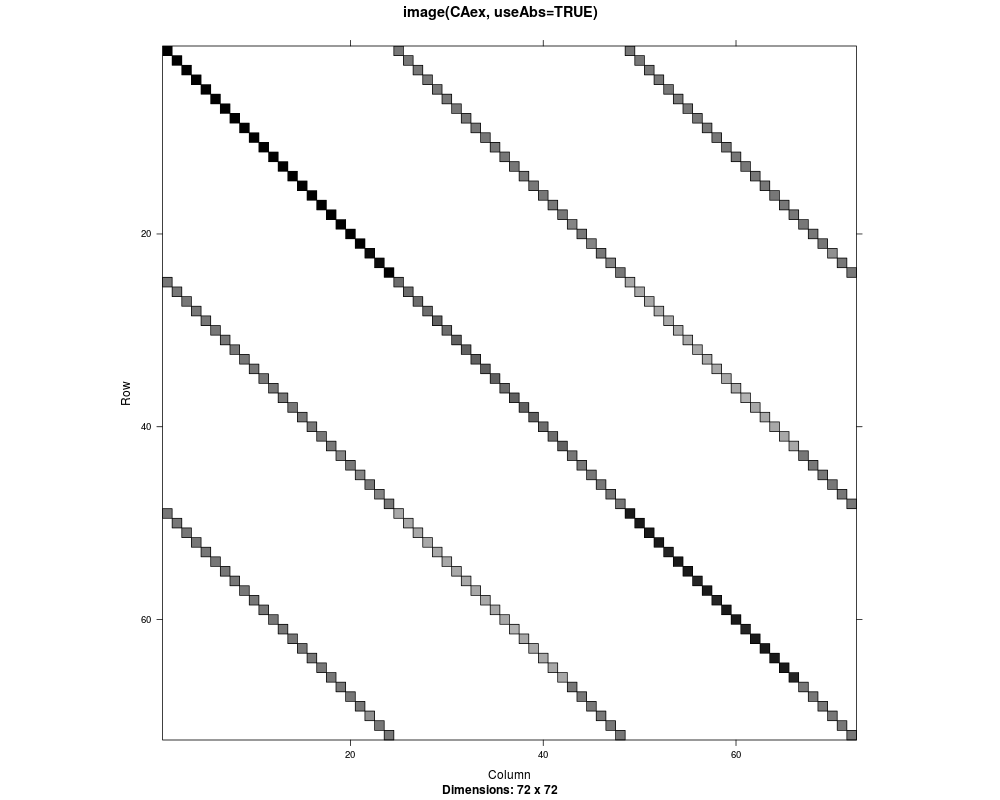
image(CAex, useAbs=TRUE, main = "image(CAex, useAbs=TRUE)")
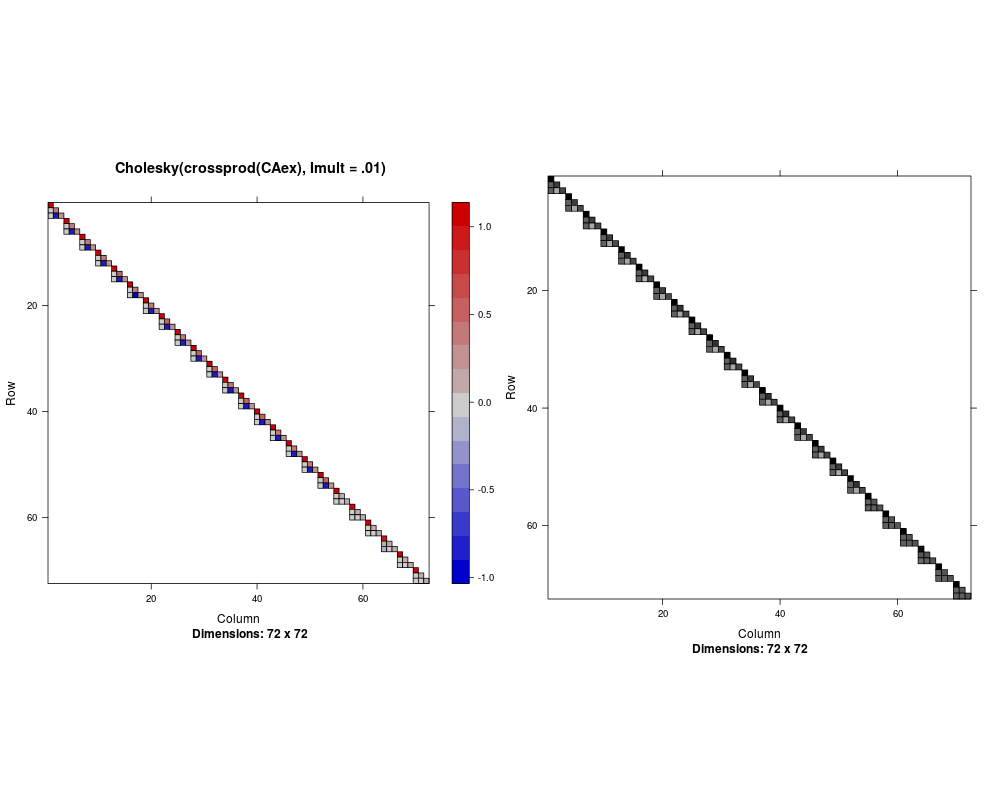
cCA <- Cholesky(crossprod(CAex), Imult = .01)
## See ?print.trellis --- place two image() plots side by side:
print(image(cCA, main="Cholesky(crossprod(CAex), Imult = .01)"),
split=c(x=1,y=1,nx=2, ny=1), more=TRUE)
print(image(cCA, useAbs=TRUE),
split=c(x=2,y=1,nx=2,ny=1))
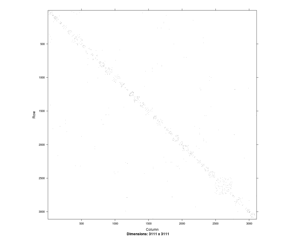
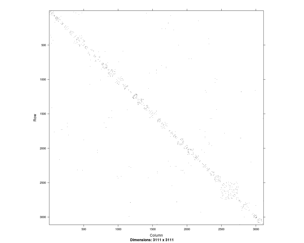
data(USCounties)
image(USCounties)# huge
image(sign(USCounties))## just the pattern
# how the result looks, may depend heavily on
# the device, screen resolution, antialiasing etc
# e.g. x11(type="Xlib") may show very differently than cairo-based
## Drawing borders around each rectangle;
# again, viewing depends very much on the device:
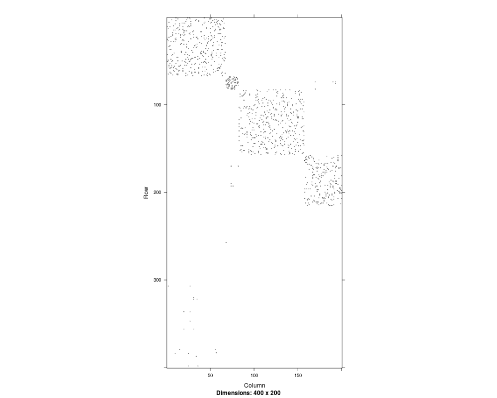
image(USCounties[1:400,1:200], lwd=.1)
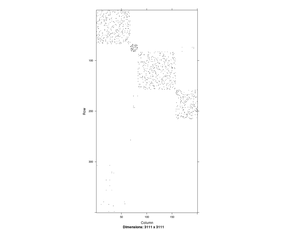
## Using (xlim,ylim) has advantage : matrix dimension and (col/row) indices:
image(USCounties, c(1,200), c(1,400), lwd=.1)
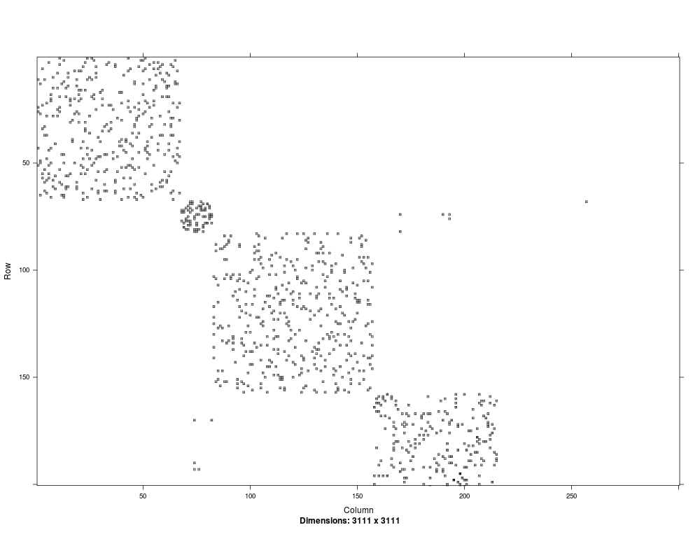
image(USCounties, c(1,300), c(1,200), lwd=.5 )
image(USCounties, c(1,300), c(1,200), lwd=.01)
if(doExtras <- interactive() || nzchar(Sys.getenv("R_MATRIX_CHECK_EXTRA")) ||
identical("true", unname(Sys.getenv("R_PKG_CHECKING_doExtras")))) {
## Using raster graphics: For PDF this would give a 77 MB file,
## however, for such a large matrix, this is typically considerably
## *slower* (than vector graphics rectangles) in most cases :
if(doPNG <- !dev.interactive())
png("image-USCounties-raster.png", width=3200, height=3200)
image(USCounties, useRaster = TRUE) # should not suffer from anti-aliasing
if(doPNG)
dev.off()
## and now look at the *.png image in a viewer you can easily zoom in and out
}#only if(doExtras)
Results
R version 3.3.1 (2016-06-21) -- "Bug in Your Hair"
Copyright (C) 2016 The R Foundation for Statistical Computing
Platform: x86_64-pc-linux-gnu (64-bit)

R is free software and comes with ABSOLUTELY NO WARRANTY.
You are welcome to redistribute it under certain conditions.
Type 'license()' or 'licence()' for distribution details.

R is a collaborative project with many contributors.
Type 'contributors()' for more information and
'citation()' on how to cite R or R packages in publications.

Type 'demo()' for some demos, 'help()' for on-line help, or
'help.start()' for an HTML browser interface to help.
Type 'q()' to quit R.

> library(Matrix)
> png(filename="/home/ddbj/snapshot/RGM3/R_CC/result/Matrix/image-methods.Rd_%03d_medium.png", width=480, height=480)
> ### Name: image-methods
> ### Title: Methods for image() in Package 'Matrix'
> ### Aliases: image-methods image,ANY-method image,CHMfactor-method
> ###   image,Matrix-method image,dgRMatrix-method image,dgCMatrix-method
> ###   image,dgTMatrix-method image,dsparseMatrix-method
> ###   image,lsparseMatrix-method image,nsparseMatrix-method
> ### Keywords: methods hplot
>
> ### ** Examples
>
> showMethods(image)
Function: image (package graphics)
x="ANY"
x="CHMfactor"
x="Matrix"
x="dgCMatrix"
x="dgRMatrix"
x="dgTMatrix"
x="dsparseMatrix"
x="lsparseMatrix"
x="nsparseMatrix"

> ## If you want to see all the methods' implementations:
> showMethods(image, incl=TRUE, inherit=FALSE)
Function: image (package graphics)
x="ANY"
function (x, ...)
UseMethod("image")


x="CHMfactor"
function (x, ...)
image(as(as(x, "sparseMatrix"), "dgTMatrix"), ...)


x="Matrix"
function (x, ...)
{
    x <- as(as(x, "sparseMatrix"), "dsparseMatrix")
    callGeneric()
}


x="dgCMatrix"
function (x, ...)
image(as(x, "dgTMatrix"), ...)


x="dgRMatrix"
function (x, ...)
image(as(x, "TsparseMatrix"), ...)


x="dgTMatrix"
function (x, ...)
{
    .local <- function (x, xlim = c(1, di[2]), ylim = c(di[1],
        1), aspect = "iso", sub = sprintf("Dimensions: %d x %d",
        di[1], di[2]), xlab = "Column", ylab = "Row", cuts = 15,
        useRaster = FALSE, useAbs = NULL, colorkey = !useAbs,
        col.regions = NULL, lwd = NULL, ...)
    {
        di <- x@Dim
        xx <- x@x
        if (missing(useAbs))
            useAbs <- min(xx, na.rm = TRUE) >= 0
        else if (useAbs)
            xx <- abs(xx)
        rx <- range(xx, finite = TRUE)
        if (is.null(col.regions))
            col.regions <- if (useAbs) {
                grey(seq(from = 0.7, to = 0, length = 100))
            }
            else {
                nn <- 100
                n0 <- min(nn, max(0, round((0 - rx[1])/(rx[2] -
                  rx[1]) * nn)))
                col.regions <- c(colorRampPalette(c("blue3",
                  "gray80"))(n0), colorRampPalette(c("gray75",
                  "red3"))(nn - n0))
            }
        if (!is.null(lwd) && !(is.numeric(lwd) && all(lwd >=
            0)))
            stop("'lwd' must be NULL or non-negative numeric")
        stopifnot(length(xlim) == 2, length(ylim) == 2)
        ylim <- sort(ylim, decreasing = TRUE)
        if (all(xlim == round(xlim)))
            xlim <- xlim + c(-0.5, +0.5)
        if (all(ylim == round(ylim)))
            ylim <- ylim + c(+0.5, -0.5)
        levelplot(x@x ~ (x@j + 1L) * (x@i + 1L), sub = sub, xlab = xlab,
            ylab = ylab, xlim = xlim, ylim = ylim, aspect = aspect,
            colorkey = colorkey, col.regions = col.regions, cuts = cuts,
            par.settings = list(background = list(col = "transparent")),
            panel = if (useRaster)
                panel.levelplot.raster
            else function(x, y, z, subscripts, at, ..., col.regions) {
                x <- as.numeric(x[subscripts])
                y <- as.numeric(y[subscripts])
                numcol <- length(at) - 1
                num.r <- length(col.regions)
                col.regions <- if (num.r <= numcol)
                  rep_len(col.regions, numcol)
                else col.regions[1 + ((1:numcol - 1) * (num.r -
                  1))%/%(numcol - 1)]
                zcol <- rep.int(NA_integer_, length(z))
                for (i in seq_along(col.regions)) zcol[!is.na(x) &
                  !is.na(y) & !is.na(z) & at[i] <= z & z < at[i +
                  1]] <- i
                zcol <- zcol[subscripts]
                if (any(subscripts)) {
                  if (is.null(lwd)) {
                    wh <- grid::current.viewport()[c("width",
                      "height")]
                    wh <- c(grid::convertWidth(wh$width, "inches",
                      valueOnly = TRUE), grid::convertHeight(wh$height,
                      "inches", valueOnly = TRUE)) * par("cra")/par("cin")
                    pSize <- wh/di
                    pA <- prod(pSize)
                    p1 <- min(pSize)
                    lwd <- if (p1 < 2 || pA < 6)
                      0.01
                    else if (p1 >= 4)
                      1
                    else if (p1 > 3)
                      0.5
                    else 0.2
                    Matrix.msg("rectangle size ", paste(round(pSize,
                      1), collapse = " x "), " [pixels];  --> lwd :",
                      formatC(lwd))
                  }
                  else stopifnot(is.numeric(lwd), all(lwd >=
                    0))
                  grid.rect(x = x, y = y, width = 1, height = 1,
                    default.units = "native", gp = gpar(fill = col.regions[zcol],
                      lwd = lwd, col = if (lwd < 0.01)
                        NA))
                }
            }, ...)
    }
    .local(x, ...)
}


x="dsparseMatrix"
function (x, ...)
image(as(x, "dgTMatrix"), ...)


x="lsparseMatrix"
function (x, ...)
image(as(x, "dMatrix"), ...)


x="nsparseMatrix"
function (x, ...)
image(as(x, "dMatrix"), ...)


>
> data(CAex)
> image(CAex, main = "image(CAex)")
> image(CAex, useAbs=TRUE, main = "image(CAex, useAbs=TRUE)")
>
> cCA <- Cholesky(crossprod(CAex), Imult = .01)
> ## See  ?print.trellis --- place two image() plots side by side:
> print(image(cCA, main="Cholesky(crossprod(CAex), Imult = .01)"),
+       split=c(x=1,y=1,nx=2, ny=1), more=TRUE)
> print(image(cCA, useAbs=TRUE),
+       split=c(x=2,y=1,nx=2,ny=1))
>
> data(USCounties)
> image(USCounties)# huge
> image(sign(USCounties))## just the pattern
>     # how the result looks, may depend heavily on
>     # the device, screen resolution, antialiasing etc
>     # e.g. x11(type="Xlib") may show very differently than cairo-based
>
> ## Drawing borders around each rectangle;
>     # again, viewing depends very much on the device:
> image(USCounties[1:400,1:200], lwd=.1)
> ## Using (xlim,ylim) has advantage : matrix dimension and (col/row) indices:
> image(USCounties, c(1,200), c(1,400), lwd=.1)
> image(USCounties, c(1,300), c(1,200), lwd=.5 )
> image(USCounties, c(1,300), c(1,200), lwd=.01)
>
> #if(doExtras <- interactive() || nzchar(Sys.getenv("R_MATRIX_CHECK_EXTRA")) ||
>     identical("true", unname(Sys.getenv("R_PKG_CHECKING_doExtras")))) {
Error: unexpected ')' in "    identical("true", unname(Sys.getenv("R_PKG_CHECKING_doExtras"))))"
Execution halted
|