Supported by Dr. Osamu Ogasawara and  . . |
|
Last data update: 2014.03.03 |
Repeat Sales EstimationDescriptionStandard and Weighted Least Squares Repeat Sales Estimation Usagerepsale(price0,time0,price1,time1,mergefirst=1, graph=TRUE,graph.conf=TRUE,conf=.95, stage3=FALSE,stage3_xlist=~timesale,print=TRUE) Arguments
DetailsThe repeat sales model is y(t) - y(s) = δ(t) - δ(s) + u(t) - u(s) where y is the log of sales price, s denotes the earlier sale in a repeat sales pair, and t denotes the later sale. Each entry of the data set should represent a repeat sales pair, with price0 = y(s), price1 = y(t), time0 = s, and time1 = t. The function repsaledata can help transfer a standard hedonic data set to a set of repeat sales pairs. Repeat sales estimates are sometimes very sensitive to sales from the first few time periods, particularly when the sample size is small. The option mergefirst indicates the number of time periods for which the price index is constrained to equal zero. The default is mergefirst = 1, meaning that the price index equals zero for just the first time period. The repsale command does not have an option for including an intercept in the model. Following Case and Shiller (1987), many authors use a three-stage procedure to construct repeat sales price indexes that are adjusted for heteroskedasticity related to the length of time between sales. Common specifications for the second-stage function are e^2 = α0 + α1 (t-s) or |e| = α0 + α1 (t-s), where e represents the first-stage residuals. The first equation implies an error variance of σ^2 = e^2 and the second equation leads to σ^2 = |e|^2. The repsale function uses a standard F test to determine whether the slope cofficients are significant in the second-stage regression. The results are reported if print=T. The third-stage equation is (y(t) - y(s))/σ = (δ(t) - δ(s))/σ + (u(t) - u(s))/σ This equation is estimated by regressing y(t) - y(s) on the series of indicator variables implied by δ(t) - δ(s) using the weights option in lm with weights = 1/sigma^2 Value
ReferencesCase, Karl and Robert Shiller, "Prices of Single-Family Homes since 1970: New Indexes for Four Cities," New England Economic Review (1987), 45-56. See Alsorepsaledata repsalefourier repsaleqreg Examplesset.seed(189) n = 2000 # sale dates range from 0-10 # drawn uniformly from all possible time0, time1 combinations with time0<time1 tmat <- expand.grid(seq(0,10), seq(0,10)) tmat <- tmat[tmat[,1]<tmat[,2], ] tobs <- sample(seq(1:nrow(tmat)),n,replace=TRUE) time0 <- tmat[tobs,1] time1 <- tmat[tobs,2] timesale <- time1-time0 table(timesale) # constant variance; index ranges from 0 at time 0 to 1 at time 10 y0 <- time0/10 + rnorm(n,0,.2) y1 <- time1/10 + rnorm(n,0,.2) fit <- repsale(price0=y0, price1=y1, time0=time0, time1=time1) # variance rises with timesale # var(u0) = .2^2; var(u1) = (.2 + timesale/10)^2 # var(u1-u0) = var(u0) + var(u1) = 2*(.2^2) + .4*timesale/10 + (timesale^2)/100 y0 <- time0/10 + rnorm(n,0,.2) y1 <- time1/10 + rnorm(n,0,.2+timesale/10) par(ask=TRUE) fit <- repsale(price0=y0, price1=y1, time0=time0, time1=time1) summary(fit$pindex) fit <- repsale(price0=y0, price1=y1, time0=time0, time1=time1, stage3="abs") summary(fit$pindex) timesale2 <- timesale^2 fit <- repsale(price0=y0, price1=y1, time0=time0, time1=time1, stage3="square", stage3_xlist=~timesale+timesale2) Results
R version 3.3.1 (2016-06-21) -- "Bug in Your Hair"
Copyright (C) 2016 The R Foundation for Statistical Computing
Platform: x86_64-pc-linux-gnu (64-bit)
R is free software and comes with ABSOLUTELY NO WARRANTY.
You are welcome to redistribute it under certain conditions.
Type 'license()' or 'licence()' for distribution details.
R is a collaborative project with many contributors.
Type 'contributors()' for more information and
'citation()' on how to cite R or R packages in publications.
Type 'demo()' for some demos, 'help()' for on-line help, or
'help.start()' for an HTML browser interface to help.
Type 'q()' to quit R.
> library(McSpatial)
Loading required package: lattice
Loading required package: locfit
locfit 1.5-9.1 2013-03-22
Loading required package: maptools
Loading required package: sp
Checking rgeos availability: TRUE
Loading required package: quantreg
Loading required package: SparseM
Attaching package: 'SparseM'
The following object is masked from 'package:base':
backsolve
Loading required package: RANN
> png(filename="/home/ddbj/snapshot/RGM3/R_CC/result/McSpatial/repsale.Rd_%03d_medium.png", width=480, height=480)
> ### Name: repsale
> ### Title: Repeat Sales Estimation
> ### Aliases: repsale
> ### Keywords: Repeat Sales
>
> ### ** Examples
>
> set.seed(189)
> n = 2000
> # sale dates range from 0-10
> # drawn uniformly from all possible time0, time1 combinations with time0<time1
> tmat <- expand.grid(seq(0,10), seq(0,10))
> tmat <- tmat[tmat[,1]<tmat[,2], ]
> tobs <- sample(seq(1:nrow(tmat)),n,replace=TRUE)
> time0 <- tmat[tobs,1]
> time1 <- tmat[tobs,2]
> timesale <- time1-time0
> table(timesale)
timesale
1 2 3 4 5 6 7 8 9 10
368 349 264 253 223 178 167 104 56 38
>
> # constant variance; index ranges from 0 at time 0 to 1 at time 10
> y0 <- time0/10 + rnorm(n,0,.2)
> y1 <- time1/10 + rnorm(n,0,.2)
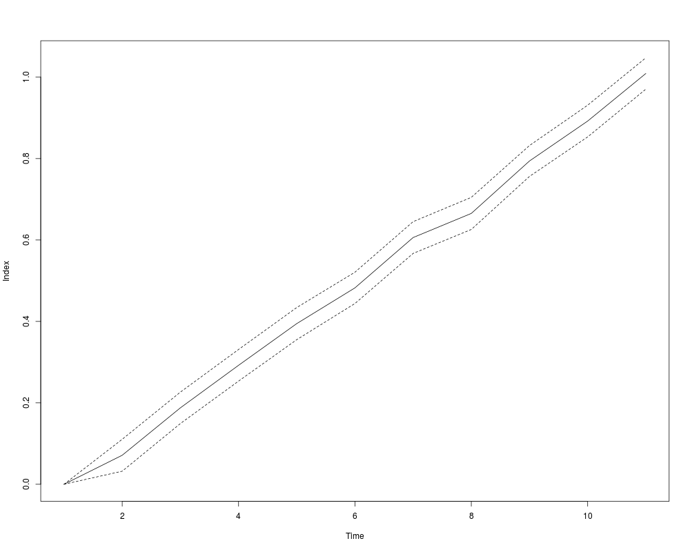
> fit <- repsale(price0=y0, price1=y1, time0=time0, time1=time1)
Call:
lm(formula = dy ~ xmat + 0)
Residuals:
Min 1Q Median 3Q Max
-0.98034 -0.18923 -0.00071 0.19144 0.90325
Coefficients:
Estimate Std. Error t value Pr(>|t|)
Time 2 0.07128 0.01999 3.567 0.00037 ***
Time 3 0.18775 0.01969 9.533 < 2e-16 ***
Time 4 0.29225 0.01981 14.753 < 2e-16 ***
Time 5 0.39466 0.02012 19.613 < 2e-16 ***
Time 6 0.48243 0.01961 24.600 < 2e-16 ***
Time 7 0.60606 0.01990 30.462 < 2e-16 ***
Time 8 0.66532 0.02010 33.104 < 2e-16 ***
Time 9 0.79412 0.01934 41.053 < 2e-16 ***
Time 10 0.89219 0.01985 44.943 < 2e-16 ***
Time 11 1.00907 0.01962 51.422 < 2e-16 ***
---
Signif. codes: 0 '***' 0.001 '**' 0.01 '*' 0.05 '.' 0.1 ' ' 1
Residual standard error: 0.2781 on 1990 degrees of freedom
Multiple R-squared: 0.742, Adjusted R-squared: 0.7407
F-statistic: 572.4 on 10 and 1990 DF, p-value: < 2.2e-16
>
> # variance rises with timesale
> # var(u0) = .2^2; var(u1) = (.2 + timesale/10)^2
> # var(u1-u0) = var(u0) + var(u1) = 2*(.2^2) + .4*timesale/10 + (timesale^2)/100
> y0 <- time0/10 + rnorm(n,0,.2)
> y1 <- time1/10 + rnorm(n,0,.2+timesale/10)
> par(ask=TRUE)
> fit <- repsale(price0=y0, price1=y1, time0=time0, time1=time1)
Call:
lm(formula = dy ~ xmat + 0)
Residuals:
Min 1Q Median 3Q Max
-3.3314 -0.4337 -0.0131 0.3928 3.0717
Coefficients:
Estimate Std. Error t value Pr(>|t|)
Time 2 0.20984 0.04976 4.217 2.59e-05 ***
Time 3 0.26246 0.04904 5.352 9.69e-08 ***
Time 4 0.36714 0.04932 7.443 1.45e-13 ***
Time 5 0.49125 0.05010 9.805 < 2e-16 ***
Time 6 0.60275 0.04883 12.344 < 2e-16 ***
Time 7 0.70359 0.04954 14.203 < 2e-16 ***
Time 8 0.85174 0.05004 17.021 < 2e-16 ***
Time 9 0.89148 0.04816 18.509 < 2e-16 ***
Time 10 0.99968 0.04943 20.224 < 2e-16 ***
Time 11 1.09254 0.04886 22.360 < 2e-16 ***
---
Signif. codes: 0 '***' 0.001 '**' 0.01 '*' 0.05 '.' 0.1 ' ' 1
Residual standard error: 0.6925 on 1990 degrees of freedom
Multiple R-squared: 0.3403, Adjusted R-squared: 0.337
F-statistic: 102.6 on 10 and 1990 DF, p-value: < 2.2e-16
> summary(fit$pindex)
Min. 1st Qu. Median Mean 3rd Qu. Max.
0.0000 0.3148 0.6027 0.5884 0.8716 1.0930
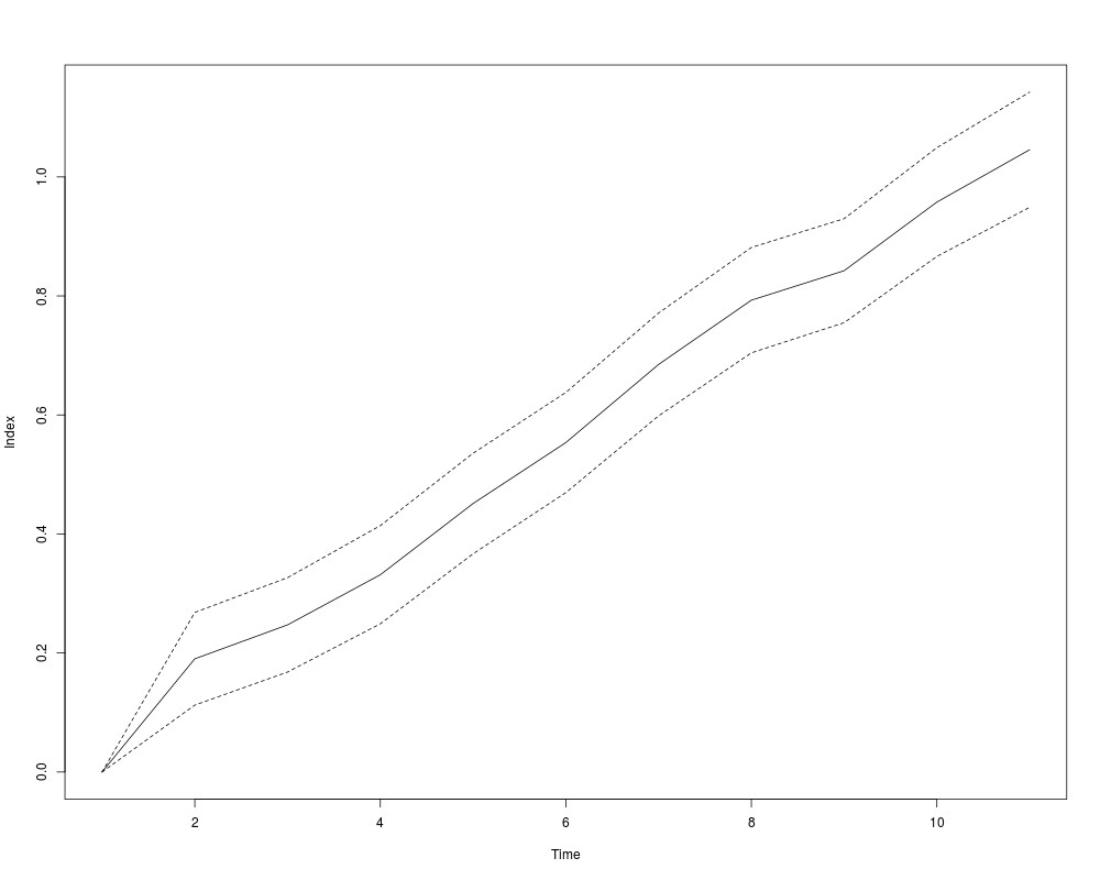
> fit <- repsale(price0=y0, price1=y1, time0=time0, time1=time1, stage3="abs")
F-value for heteroskedasticity test = 415.8353
p-value = 1
Call:
lm(formula = dy ~ xmat + 0, weights = wgt)
Weighted Residuals:
Min 1Q Median 3Q Max
-4.8921 -0.8596 -0.0084 0.8311 3.8085
Coefficients:
Estimate Std. Error t value Pr(>|t|)
Time 2 0.19027 0.03970 4.792 1.77e-06 ***
Time 3 0.24730 0.04043 6.117 1.14e-09 ***
Time 4 0.33152 0.04206 7.882 5.27e-15 ***
Time 5 0.45119 0.04308 10.472 < 2e-16 ***
Time 6 0.55364 0.04291 12.902 < 2e-16 ***
Time 7 0.68489 0.04405 15.547 < 2e-16 ***
Time 8 0.79288 0.04514 17.563 < 2e-16 ***
Time 9 0.84239 0.04455 18.908 < 2e-16 ***
Time 10 0.95772 0.04661 20.550 < 2e-16 ***
Time 11 1.04569 0.04934 21.195 < 2e-16 ***
---
Signif. codes: 0 '***' 0.001 '**' 0.01 '*' 0.05 '.' 0.1 ' ' 1
Residual standard error: 1.247 on 1990 degrees of freedom
Multiple R-squared: 0.2605, Adjusted R-squared: 0.2568
F-statistic: 70.11 on 10 and 1990 DF, p-value: < 2.2e-16
> summary(fit$pindex)
Min. 1st Qu. Median Mean 3rd Qu. Max.
0.0000 0.2894 0.5536 0.5543 0.8176 1.0460
> timesale2 <- timesale^2
> fit <- repsale(price0=y0, price1=y1, time0=time0, time1=time1, stage3="square",
+ stage3_xlist=~timesale+timesale2)
F-value for heteroskedasticity test = 185.2463
p-value = 1
Call:
lm(formula = dy ~ xmat + 0, weights = wgt)
Weighted Residuals:
Min 1Q Median 3Q Max
-3.9776 -0.6828 -0.0080 0.6746 2.8256
Coefficients:
Estimate Std. Error t value Pr(>|t|)
Time 2 0.18887 0.04096 4.611 4.26e-06 ***
Time 3 0.24581 0.04088 6.014 2.15e-09 ***
Time 4 0.33034 0.04228 7.813 8.98e-15 ***
Time 5 0.45061 0.04316 10.441 < 2e-16 ***
Time 6 0.55518 0.04297 12.921 < 2e-16 ***
Time 7 0.67922 0.04413 15.391 < 2e-16 ***
Time 8 0.79412 0.04532 17.524 < 2e-16 ***
Time 9 0.83978 0.04472 18.778 < 2e-16 ***
Time 10 0.95210 0.04692 20.293 < 2e-16 ***
Time 11 1.04344 0.04950 21.078 < 2e-16 ***
---
Signif. codes: 0 '***' 0.001 '**' 0.01 '*' 0.05 '.' 0.1 ' ' 1
Residual standard error: 0.9989 on 1990 degrees of freedom
Multiple R-squared: 0.2633, Adjusted R-squared: 0.2596
F-statistic: 71.14 on 10 and 1990 DF, p-value: < 2.2e-16
>
>
>
>
>
> dev.off()
null device
1
>
|