R Graphical Manual

Browse All

Last data update: 2014.03.03

R: Repeat Sales Estimation using Fourier Expansions

repsalefourier

R Documentation

Repeat Sales Estimation using Fourier Expansions

Description

Standard and Weighted Least Squares Repeat Sales Estimation using Fourier Expansions

Usage

repsalefourier(price0,time0,price1,time1,mergefirst=1,q=1, graph=TRUE,
  graph.conf=TRUE,conf=.95,stage3=FALSE,stage3_xlist=~timesale,
  print=TRUE)

Arguments

`price0`	Earlier price in repeat sales pair
`time0`	Earlier time in repeat sales pair
`price1`	Later price in repeat sales pair
`time1`	Later time in repeat sales pair
`mergefirst`	Number of initial periods with coefficients constrained to zero. Default: mergefirst=1
`q`	Sets Q for the fourier expansion. Default: q=1.
`graph`	If TRUE, graph results. Default: graph=T
`graph.conf`	If TRUE, add confidence intervals to graph. Default: graph.conf=T
`conf`	Confidence level for intervals. Default: .95
`stage3`	If stage3 = NULL, no corrections for heteroskedasticty. If stage3="abs", uses the absolute value of the first-stage residuals as the dependent variable in the second-stage regression. If stage3="square", uses the square of the first-stage residuals as the dependent variable. Default: stage3=NULL.
`stage3_xlist`	List of explanatory variables for heteroskedasticity. By default, the single variable timesale = time1-time0 is constructed and used as the explanatory variable when stage3="abs" or stage3="square". Alternatively, a formula can be provided for a user-specified list of explanatory variables, e.g., stage3_xlist=~x1+x2. Important: note the "~" before the variable list.
`print`	If print=T, prints the regression results. Prints one stage only – the first stage when stage=NULL and the final stage when stage3="square" or stage3="abs". Default: print=T.

Details

The repeat sales model is

y(t) - y(s) = δ(t) - δ(s) + u(t) - u(s)

where y is the log of sale price, s denotes the earlier sale in a repeat sales pair, and t denotes the later sale. Each entry of the data set should represent a repeat sales pair, with price0 = y(s), price1 = y(t), time0 = s, and time1 = t. The function repsaledata can help transfer a standard hedonic data set to a set of repeat sales pairs.

The repeat sales model can be derived from a hedonic price function with the form y_{i,t} = δ_t + X_i β + u_{i,t} where X_i is a vector of variables that are assumed constant over time. repsalefourier replaces δ_t with a smooth continuous function, g(T_i) where T_i denotes the time of sale for observation i. Letting g(T_i) = α_0 + α_1 z_i + α_2 z_i^2 + ∑_{i=1}^Q {λ_q sin(qz_i) + γ_q cos(qz_i) } , where z_i = 2 π (T_i - min(T_i))/(max(T_i) - min(T_i)) , the repeat sales model becomes y_{i,t} - y_{i,s} = g(T_i) - g(T_i^s) =

α_1 (z_i - z_i^s) + α_2 (z_i^2 - z_i^{s2}) + ∑_{q=1}^Q { λ_q (sin(qz_i) - sin(qz_i^s)) + γ_q (cos(qz_i) - cos(z_i^s)) } + u_{i,t} - u_{i,t-s}

After imposing the constraint that the price index in the base time period equals zero, the index is constructed from the estimated regression using the following expression:

g(T_i) = α_1 z_i + α_2 z_i^2 + ∑_{q=1}^Q { λ_q sin(qz_i) + γ_q (cos(qz_i) - 1) }

More details can be found in McMillen and Dombrow (2001).

Repeat sales estimates are sometimes very sensitive to sales from the first few time periods, particularly when the sample size is small. The option mergefirst indicates the number of time periods for which the price index is constrained to equal zero. The default is mergefirst = 1, meaning that the price index equals zero for just the first time period. The repsalefourier command does not have an option for including an intercept in the model.

Following Case and Shiller (1987), many authors use a three-stage procedure to construct repeat sales price indexes that are adjusted for heteroskedasticity related to the length of time between sales. Common specifications for the second-stage function are e^2 = α0 + α1 (t-s) or |e| = α0 + α1 (t-s), where e represents the first-stage residuals. The first equation implies an error variance of σ^2 = e^2 and the second equation leads to σ^2 = |e|^2. The repsalefourier function uses a standard F test to determine whether the slope cofficients are significant in the second-stage regression. The results are reported if print=T.

The third-stage equation is

(y(t) - y(s))/σ = (g(T) - g(T_s))/σ + (u(t) - u(s))/σ

This equation is estimated by regressing y(t) - y(s) on z, z^2, sin(z)...sin(Qz), cos(z)...cos(Qz) using the weights option in lm with weights = 1/sigma^2

Value

`fit`	Full regression model.
`pindex`	The estimated price index.
`lo`	The lower bounds for the price index confidence intervals.
`hi`	The upper bounds for the price index confidence intervals.
`dy`	The dependent variable for the repeat sales regression, dy = price1-price0.
`xmat`	The matrix of explanatory variables for the repeat sales regressions. dim(xmat) = 2 + 2Q.

References

Case, Karl and Robert Shiller, "Prices of Single-Family Homes since 1970: New Indexes for Four Cities," New England Economic Review (1987), 45-56.

McMillen, Daniel P. and Jonathan Dombrow, "A Flexible Fourier Approach to Repeat Sales Price Indexes," Real Estate Economics 29 (2001), 207-225.

Examples

set.seed(189)
n = 2000
# sale dates range from 0-50
# drawn uniformly from all possible time0, time1 combinations with time0<time1
tmat <- expand.grid(seq(0,50), seq(0,50))
tmat <- tmat[tmat[,1]<tmat[,2], ]
tobs <- sample(seq(1:nrow(tmat)),n,replace=TRUE)
time0 <- tmat[tobs,1]
time1 <- tmat[tobs,2]
timesale <- time1-time0
timesale2 <- timesale^2

par(ask=TRUE)
z0 <- 2*pi*time0/50
z0sq <- z0^2
sin0 <- sin(z0)
cos0 <- cos(z0)
z1 <- 2*pi*time1/50
z1sq <- z1^2
sin1 <- sin(z1)
cos1 <- cos(z1)
ybase0 <- z0 + .05*z0sq -.5*sin0 - .5*cos0
miny <- min(ybase0)
ybase0 <- ybase0-miny
ybase1 <- z1 + .05*z1sq -.5*sin1 - .5*cos1 - miny
maxy <- max(ybase1)
ybase0 <- ybase0/maxy
ybase1 <- ybase1/maxy
summary(data.frame(ybase0,ybase1))
sig1 = sd(c(ybase0,ybase1))/2
y0 <- ybase0 + rnorm(n,0,sig1)
y1 <- ybase1 + rnorm(n,0,sig1)
fit <- lm(y0~z0+z0sq+sin0+cos0)
summary(fit)
plot(time0,fitted(fit))
fit <- lm(y1~z1+z1sq+sin1+cos1)
summary(fit)
plot(time1,fitted(fit))

fit1 <- repsale(price1=y1,price0=y0,time1=time1,time0=time0,graph=FALSE,
  mergefirst=5)
fit2 <- repsalefourier(price1=y1,price0=y0,time1=time1,time0=time0,q=1,
  graph=FALSE,mergefirst=5)
timevar <- seq(0,50)
plot(timevar,fit1$pindex,type="l",xlab="Time",ylab="Index",
  ylim=c(min(fit1$pindex),max(fit2$pindex)))
lines(timevar,fit2$pindex)



# variance rises with timesale
# var(u0) = sig1^2; var(u1) = (sig1 + timesale/50)^2
# var(u1-u0) = var(u0) + var(u1) = 2*(sig1^2) + 2*sig1*timesale/10 + (timesale^2)/2500
y0 <- ybase0 + rnorm(n,0,sig1)
y1 <- ybase1 + rnorm(n,0,sig1+timesale/50)
par(ask=TRUE)
fit1 <- repsalefourier(price0=y0, price1=y1, time0=time0, time1=time1,
  graph=FALSE)
fit2 <- repsalefourier(price0=y0, price1=y1, time0=time0, time1=time1,
  graph=FALSE,stage3="abs",stage3_xlist=~timesale+timesale2)
plot(timevar,fit1$lo,type="l",xlab="Time",ylab="Index",
  ylim=c(min(fit1$lo,fit2$lo),max(fit1$hi,fit2$hi)))
lines(timevar,fit1$hi)
lines(timevar,fit2$lo,col="red")
lines(timevar,fit2$hi,col="red")

Results


R version 3.3.1 (2016-06-21) -- "Bug in Your Hair"
Copyright (C) 2016 The R Foundation for Statistical Computing
Platform: x86_64-pc-linux-gnu (64-bit)

R is free software and comes with ABSOLUTELY NO WARRANTY.
You are welcome to redistribute it under certain conditions.
Type 'license()' or 'licence()' for distribution details.

R is a collaborative project with many contributors.
Type 'contributors()' for more information and
'citation()' on how to cite R or R packages in publications.

Type 'demo()' for some demos, 'help()' for on-line help, or
'help.start()' for an HTML browser interface to help.
Type 'q()' to quit R.

> library(McSpatial)
Loading required package: lattice
Loading required package: locfit
locfit 1.5-9.1 	 2013-03-22
Loading required package: maptools
Loading required package: sp
Checking rgeos availability: TRUE
Loading required package: quantreg
Loading required package: SparseM

Attaching package: 'SparseM'

The following object is masked from 'package:base':

    backsolve

Loading required package: RANN
> png(filename="/home/ddbj/snapshot/RGM3/R_CC/result/McSpatial/repsalefourier.Rd_%03d_medium.png", width=480, height=480)
> ### Name: repsalefourier
> ### Title: Repeat Sales Estimation using Fourier Expansions
> ### Aliases: repsalefourier
> ### Keywords: Repeat Sales Series Expansions
> 
> ### ** Examples
> 
> set.seed(189)
> n = 2000
> # sale dates range from 0-50
> # drawn uniformly from all possible time0, time1 combinations with time0<time1
> tmat <- expand.grid(seq(0,50), seq(0,50))
> tmat <- tmat[tmat[,1]<tmat[,2], ]
> tobs <- sample(seq(1:nrow(tmat)),n,replace=TRUE)
> time0 <- tmat[tobs,1]
> time1 <- tmat[tobs,2]
> timesale <- time1-time0
> timesale2 <- timesale^2
> 
> par(ask=TRUE)
> z0 <- 2*pi*time0/50
> z0sq <- z0^2
> sin0 <- sin(z0)
> cos0 <- cos(z0)
> z1 <- 2*pi*time1/50
> z1sq <- z1^2
> sin1 <- sin(z1)
> cos1 <- cos(z1)
> ybase0 <- z0 + .05*z0sq -.5*sin0 - .5*cos0
> miny <- min(ybase0)
> ybase0 <- ybase0-miny
> ybase1 <- z1 + .05*z1sq -.5*sin1 - .5*cos1 - miny
> maxy <- max(ybase1)
> ybase0 <- ybase0/maxy
> ybase1 <- ybase1/maxy
> summary(data.frame(ybase0,ybase1))
     ybase0            ybase1       
 Min.   :0.00000   Min.   :0.01766  
 1st Qu.:0.06972   1st Qu.:0.58855  
 Median :0.24423   Median :0.81880  
 Mean   :0.32742   Mean   :0.71910  
 3rd Qu.:0.53337   3rd Qu.:0.91262  
 Max.   :0.98338   Max.   :1.00000  
> sig1 = sd(c(ybase0,ybase1))/2
> y0 <- ybase0 + rnorm(n,0,sig1)
> y1 <- ybase1 + rnorm(n,0,sig1)
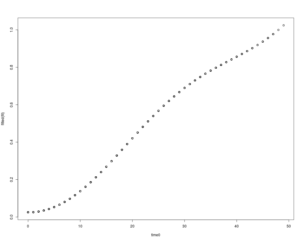
> fit <- lm(y0~z0+z0sq+sin0+cos0)
> summary(fit)

Call:
lm(formula = y0 ~ z0 + z0sq + sin0 + cos0)

Residuals:
     Min       1Q   Median       3Q      Max 
-0.46899 -0.11088  0.00102  0.10987  0.55996 

Coefficients:
             Estimate Std. Error t value Pr(>|t|)    
(Intercept)  0.126480   0.029869   4.235 2.39e-05 ***
z0           0.052986   0.033681   1.573  0.11584    
z0sq         0.017544   0.006042   2.904  0.00373 ** 
sin0        -0.054164   0.012599  -4.299 1.80e-05 ***
cos0        -0.101442   0.021464  -4.726 2.45e-06 ***
---
Signif. codes:  0 '***' 0.001 '**' 0.01 '*' 0.05 '.' 0.1 ' ' 1

Residual standard error: 0.1621 on 1995 degrees of freedom
Multiple R-squared:  0.7489,	Adjusted R-squared:  0.7484 
F-statistic:  1487 on 4 and 1995 DF,  p-value: < 2.2e-16

> plot(time0,fitted(fit))
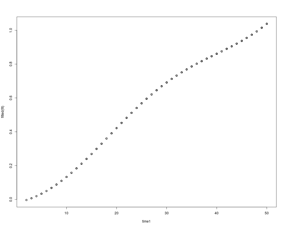
> fit <- lm(y1~z1+z1sq+sin1+cos1)
> summary(fit)

Call:
lm(formula = y1 ~ z1 + z1sq + sin1 + cos1)

Residuals:
     Min       1Q   Median       3Q      Max 
-0.53279 -0.11361  0.00073  0.11066  0.56063 

Coefficients:
             Estimate Std. Error t value Pr(>|t|)    
(Intercept)  0.066206   0.062896   1.053 0.292642    
z1           0.097339   0.045591   2.135 0.032879 *  
z1sq         0.011277   0.006403   1.761 0.078365 .  
sin1        -0.049476   0.013680  -3.617 0.000306 ***
cos1        -0.085123   0.022339  -3.811 0.000143 ***
---
Signif. codes:  0 '***' 0.001 '**' 0.01 '*' 0.05 '.' 0.1 ' ' 1

Residual standard error: 0.1665 on 1995 degrees of freedom
Multiple R-squared:  0.7127,	Adjusted R-squared:  0.7121 
F-statistic:  1237 on 4 and 1995 DF,  p-value: < 2.2e-16

> plot(time1,fitted(fit))
> 
> fit1 <- repsale(price1=y1,price0=y0,time1=time1,time0=time0,graph=FALSE,
+   mergefirst=5)

Call:
lm(formula = dy ~ xmat + 0)

Residuals:
     Min       1Q   Median       3Q      Max 
-0.76791 -0.15748 -0.00397  0.14970  0.76721 

Coefficients:
        Estimate Std. Error t value Pr(>|t|)    
Time 6   0.05741    0.02860   2.007 0.044860 *  
Time 7   0.02809    0.02881   0.975 0.329652    
Time 8   0.07619    0.02834   2.688 0.007240 ** 
Time 9   0.10328    0.02664   3.877 0.000109 ***
Time 10  0.11611    0.02858   4.063 5.05e-05 ***
Time 11  0.12408    0.02939   4.223 2.53e-05 ***
Time 12  0.17446    0.02719   6.416 1.75e-10 ***
Time 13  0.14583    0.02836   5.142 3.00e-07 ***
Time 14  0.20087    0.02746   7.315 3.73e-13 ***
Time 15  0.21490    0.02943   7.301 4.13e-13 ***
Time 16  0.23677    0.02787   8.497  < 2e-16 ***
Time 17  0.32424    0.02677  12.113  < 2e-16 ***
Time 18  0.31677    0.02797  11.325  < 2e-16 ***
Time 19  0.30955    0.02992  10.347  < 2e-16 ***
Time 20  0.42779    0.02951  14.496  < 2e-16 ***
Time 21  0.40472    0.03106  13.032  < 2e-16 ***
Time 22  0.41121    0.02844  14.457  < 2e-16 ***
Time 23  0.48181    0.02746  17.546  < 2e-16 ***
Time 24  0.45078    0.02792  16.146  < 2e-16 ***
Time 25  0.54754    0.03002  18.240  < 2e-16 ***
Time 26  0.54222    0.02950  18.382  < 2e-16 ***
Time 27  0.55827    0.02995  18.643  < 2e-16 ***
Time 28  0.61153    0.02772  22.058  < 2e-16 ***
Time 29  0.65244    0.03033  21.512  < 2e-16 ***
Time 30  0.67971    0.02963  22.936  < 2e-16 ***
Time 31  0.65930    0.02859  23.064  < 2e-16 ***
Time 32  0.69045    0.02967  23.268  < 2e-16 ***
Time 33  0.73335    0.02935  24.985  < 2e-16 ***
Time 34  0.71458    0.02784  25.666  < 2e-16 ***
Time 35  0.69007    0.02876  23.991  < 2e-16 ***
Time 36  0.79646    0.02681  29.703  < 2e-16 ***
Time 37  0.78707    0.03031  25.968  < 2e-16 ***
Time 38  0.81238    0.02665  30.480  < 2e-16 ***
Time 39  0.85246    0.02847  29.940  < 2e-16 ***
Time 40  0.84563    0.02729  30.991  < 2e-16 ***
Time 41  0.84820    0.02801  30.277  < 2e-16 ***
Time 42  0.88384    0.02943  30.028  < 2e-16 ***
Time 43  0.85156    0.02878  29.584  < 2e-16 ***
Time 44  0.86039    0.02856  30.125  < 2e-16 ***
Time 45  0.93503    0.02803  33.356  < 2e-16 ***
Time 46  0.92738    0.02669  34.745  < 2e-16 ***
Time 47  0.92690    0.02774  33.418  < 2e-16 ***
Time 48  0.95810    0.02707  35.399  < 2e-16 ***
Time 49  0.98146    0.02731  35.939  < 2e-16 ***
Time 50  0.96114    0.02964  32.423  < 2e-16 ***
Time 51  1.04543    0.02733  38.259  < 2e-16 ***
---
Signif. codes:  0 '***' 0.001 '**' 0.01 '*' 0.05 '.' 0.1 ' ' 1

Residual standard error: 0.2303 on 1954 degrees of freedom
Multiple R-squared:  0.8205,	Adjusted R-squared:  0.8162 
F-statistic: 194.1 on 46 and 1954 DF,  p-value: < 2.2e-16

> fit2 <- repsalefourier(price1=y1,price0=y0,time1=time1,time0=time0,q=1,
+   graph=FALSE,mergefirst=5)

Call:
lm(formula = dy ~ xmat + 0)

Residuals:
     Min       1Q   Median       3Q      Max 
-0.82133 -0.16028 -0.00466  0.15482  0.75944 

Coefficients:
          Estimate Std. Error t value Pr(>|t|)    
dz        0.086426   0.021788   3.967 7.55e-05 ***
dzsq      0.012088   0.003562   3.393 0.000704 ***
dsin(1z) -0.056430   0.007327  -7.702 2.09e-14 ***
dcos(1z) -0.079129   0.016125  -4.907 9.99e-07 ***
---
Signif. codes:  0 '***' 0.001 '**' 0.01 '*' 0.05 '.' 0.1 ' ' 1

Residual standard error: 0.2301 on 1996 degrees of freedom
Multiple R-squared:  0.8168,	Adjusted R-squared:  0.8164 
F-statistic:  2225 on 4 and 1996 DF,  p-value: < 2.2e-16

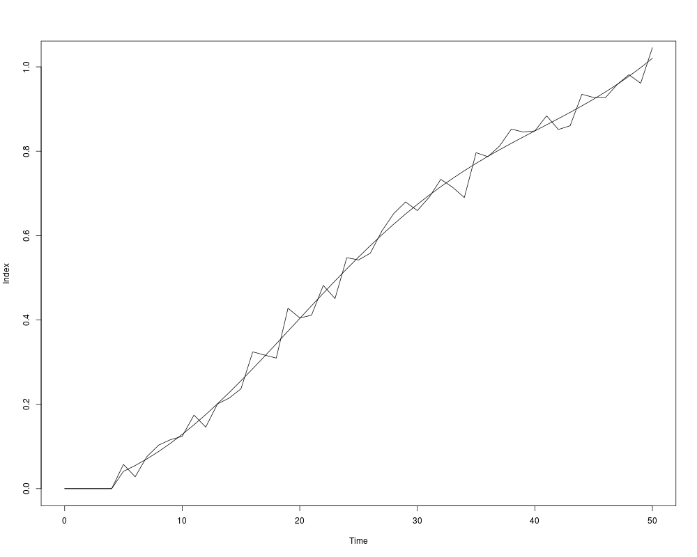
> timevar <- seq(0,50)
> plot(timevar,fit1$pindex,type="l",xlab="Time",ylab="Index",
+   ylim=c(min(fit1$pindex),max(fit2$pindex)))
> lines(timevar,fit2$pindex)
> 
> 
> 
> # variance rises with timesale
> # var(u0) = sig1^2; var(u1) = (sig1 + timesale/50)^2
> # var(u1-u0) = var(u0) + var(u1) = 2*(sig1^2) + 2*sig1*timesale/10 + (timesale^2)/2500
> y0 <- ybase0 + rnorm(n,0,sig1)
> y1 <- ybase1 + rnorm(n,0,sig1+timesale/50)
> par(ask=TRUE)
> fit1 <- repsalefourier(price0=y0, price1=y1, time0=time0, time1=time1,
+   graph=FALSE)

Call:
lm(formula = dy ~ xmat + 0)

Residuals:
    Min      1Q  Median      3Q     Max 
-3.1965 -0.3373  0.0067  0.3468  2.1758 

Coefficients:
          Estimate Std. Error t value Pr(>|t|)    
dz        0.115576   0.069150   1.671   0.0948 .  
dzsq      0.006168   0.010909   0.565   0.5719    
dsin(1z) -0.081898   0.020915  -3.916 9.32e-05 ***
dcos(1z) -0.071968   0.046635  -1.543   0.1229    
---
Signif. codes:  0 '***' 0.001 '**' 0.01 '*' 0.05 '.' 0.1 ' ' 1

Residual standard error: 0.618 on 1996 degrees of freedom
Multiple R-squared:  0.3797,	Adjusted R-squared:  0.3785 
F-statistic: 305.5 on 4 and 1996 DF,  p-value: < 2.2e-16

> fit2 <- repsalefourier(price0=y0, price1=y1, time0=time0, time1=time1,
+   graph=FALSE,stage3="abs",stage3_xlist=~timesale+timesale2)
F-value for heteroskedasticity test =  301.6005 
p-value =  1 

Call:
lm(formula = dy ~ xmat + 0, weights = wgt)

Weighted Residuals:
    Min      1Q  Median      3Q     Max 
-4.7727 -0.8578  0.0099  0.8443  3.8578 

Coefficients:
          Estimate Std. Error t value Pr(>|t|)    
dz        0.135092   0.056093   2.408   0.0161 *  
dzsq      0.003459   0.008834   0.392   0.6954    
dsin(1z) -0.075015   0.017315  -4.332 1.55e-05 ***
dcos(1z) -0.054409   0.036713  -1.482   0.1385    
---
Signif. codes:  0 '***' 0.001 '**' 0.01 '*' 0.05 '.' 0.1 ' ' 1

Residual standard error: 1.239 on 1996 degrees of freedom
Multiple R-squared:  0.3086,	Adjusted R-squared:  0.3072 
F-statistic: 222.7 on 4 and 1996 DF,  p-value: < 2.2e-16

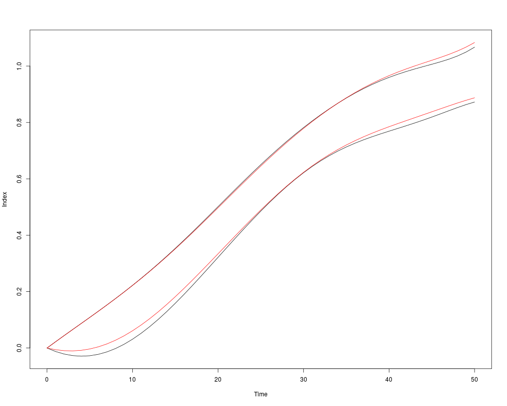
> plot(timevar,fit1$lo,type="l",xlab="Time",ylab="Index",
+   ylim=c(min(fit1$lo,fit2$lo),max(fit1$hi,fit2$hi)))
> lines(timevar,fit1$hi)
> lines(timevar,fit2$lo,col="red")
> lines(timevar,fit2$hi,col="red")
> 
> 
> 
> 
> 
> 
> dev.off()
null device 
          1 
>