Univariate or Bivariate Interpolation

Description

Uses the Akima (1970) method for univariate interpolation and the Modified Shephard Algorithm for bivariate interpolation.

Usage

 smooth12(x,y,xout,knum=16,std=TRUE) 

Arguments

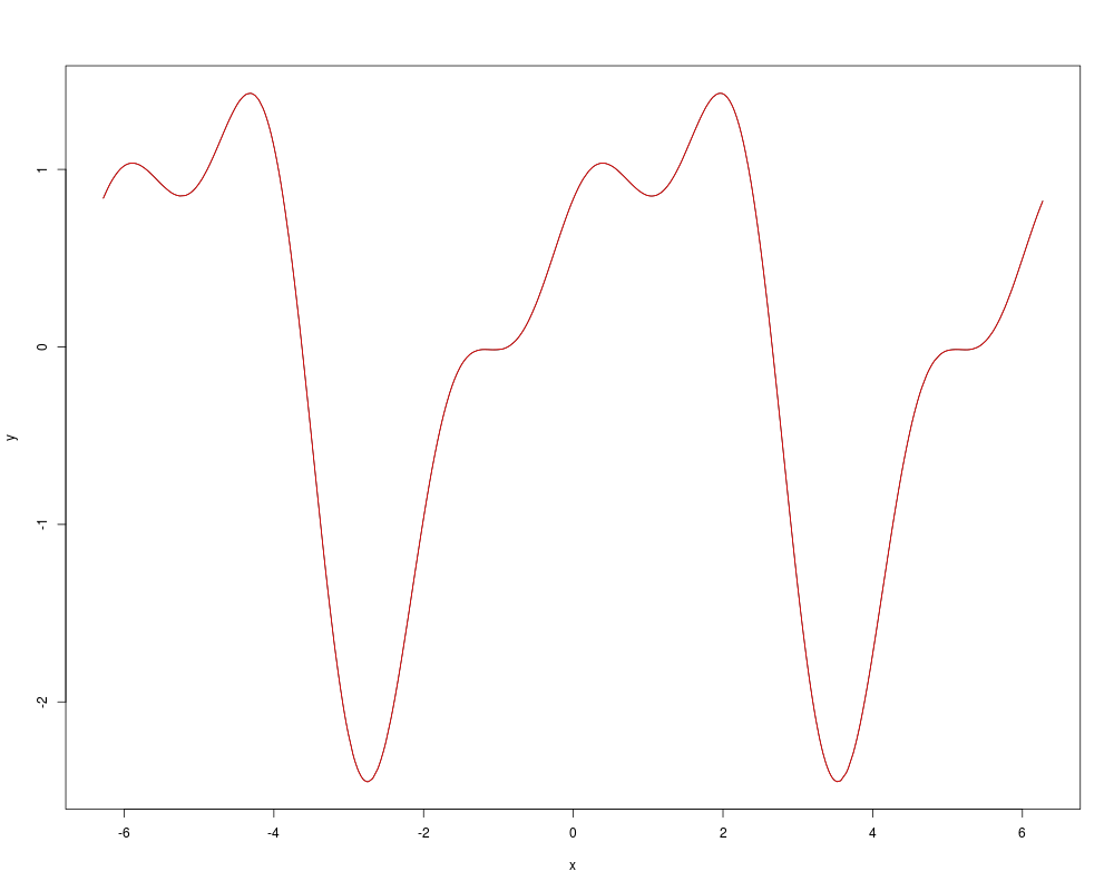
Details

The univariate version of the function is designed as a partial replacement for the aspline function in the akima package. It produces a smooth function that closely resembles the interpolation that would be done by hand. Values of y are averaged across any ties for x. The function does not allow for extrapolation beyond the min(x), max(x) range.

The bivariate version of the function uses the modifed Shepard's method for interpolation. The function uses the RANN package to find the nearest knum target points to each location in xout. The following formula is used to interpolate from these target points to the locations given in xout:

frac{∑_{i=1}^{knum} w_i y_i}{∑_{i=1}^{knum} w_i}

where

w_{i} = ((maxd - d_{i})^2)/(maxd*d_{i})

and

maxd = max(d_{1}, ..., d_{knum}).

Value

The values of y interpolated to the xout locations.

References

Akima, Hiroshi, "A New Method of Interpolation and Smooth Curve Fitting Based on Local Procedures," Journal of the Association for Computing Machinery 17 (1970), 589-602.

Franke, R. and G. Neilson, "Smooth Interpolation of Large Sets of Scatter data," International Journal of Numerical Methods in Engineering 15 (1980), 1691 - 1704.

See Also

maketarget

Examples

set.seed(484849)
n = 1000
x <- runif(n,-2*pi,2*pi)
x <- sort(x)
y <- sin(x) + cos(x) - .5*sin(2*x) - .5*cos(2*x) + sin(3*x)/3 + cos(3*x)/3
x1 <- seq(-2*pi,2*pi,length=100)
y1 <- sin(x1) + cos(x1) - .5*sin(2*x1) - .5*cos(2*x1) + sin(3*x1)/3 + cos(3*x1)/3

yout <- smooth12(x1,y1,x)
plot(x,y,type="l")
lines(x,yout,col="red")

x <- seq(0,10)
xmat <- expand.grid(x,x)
y <- sqrt((xmat[,1]-5)^2 + (xmat[,2]-5)^2)
xout <- cbind(runif(n,0,10),runif(n,0,10))
y1 <- sqrt((xout[,1]-5)^2 + (xout[,2]-5)^2)
y2 <- smooth12(xmat,y,xout)
cor(y1,y2)

Results

R version 3.3.1 (2016-06-21) -- "Bug in Your Hair"
Copyright (C) 2016 The R Foundation for Statistical Computing
Platform: x86_64-pc-linux-gnu (64-bit)

R is free software and comes with ABSOLUTELY NO WARRANTY.
You are welcome to redistribute it under certain conditions.
Type 'license()' or 'licence()' for distribution details.

R is a collaborative project with many contributors.
Type 'contributors()' for more information and
'citation()' on how to cite R or R packages in publications.

Type 'demo()' for some demos, 'help()' for on-line help, or
'help.start()' for an HTML browser interface to help.
Type 'q()' to quit R.

> library(McSpatial)
Loading required package: lattice
Loading required package: locfit
locfit 1.5-9.1 	 2013-03-22
Loading required package: maptools
Loading required package: sp
Checking rgeos availability: TRUE
Loading required package: quantreg
Loading required package: SparseM

Attaching package: 'SparseM'

The following object is masked from 'package:base':

    backsolve

Loading required package: RANN
> png(filename="/home/ddbj/snapshot/RGM3/R_CC/result/McSpatial/smooth12.Rd_%03d_medium.png", width=480, height=480)
> ### Name: smooth12
> ### Title: Univariate or Bivariate Interpolation
> ### Aliases: smooth12
> 
> ### ** Examples
> 
> set.seed(484849)
> n = 1000
> x <- runif(n,-2*pi,2*pi)
> x <- sort(x)
> y <- sin(x) + cos(x) - .5*sin(2*x) - .5*cos(2*x) + sin(3*x)/3 + cos(3*x)/3
> x1 <- seq(-2*pi,2*pi,length=100)
> y1 <- sin(x1) + cos(x1) - .5*sin(2*x1) - .5*cos(2*x1) + sin(3*x1)/3 + cos(3*x1)/3
> 
> yout <- smooth12(x1,y1,x)
> plot(x,y,type="l")
> lines(x,yout,col="red")
> 
> x <- seq(0,10)
> xmat <- expand.grid(x,x)
> y <- sqrt((xmat[,1]-5)^2 + (xmat[,2]-5)^2)
> xout <- cbind(runif(n,0,10),runif(n,0,10))
> y1 <- sqrt((xout[,1]-5)^2 + (xout[,2]-5)^2)
> y2 <- smooth12(xmat,y,xout)
> cor(y1,y2)
[1] 0.9989234
> 
> 
> 
> 
> 
> dev.off()
null device 
          1 
>