Normal Laplace Distribution

Description

Density function, distribution function, quantiles and random number generation for the normal Laplace distribution, with parameters mu (location), delta (scale), beta (skewness), and nu (shape).

Usage

dnl(x, mu = 0, sigma = 1, alpha = 1, beta = 1,
    param = c(mu,sigma,alpha,beta))
pnl(q, mu = 0, sigma = 1, alpha = 1, beta = 1,
    param = c(mu,sigma,alpha,beta))
qnl(p, mu = 0, sigma = 1, alpha = 1, beta = 1,
    param = c(mu,sigma,alpha,beta),
    tol = 10^(-5), nInterpol = 100, subdivisions = 100, ...)
rnl(n, mu = 0, sigma = 1, alpha = 1, beta = 1,
    param = c(mu,sigma,alpha,beta))

Arguments

Details

Users may either specify the values of the parameters individually or as a vector. If both forms are specified, then the values specified by the vector param will overwrite the other ones.

The density function is

f(y) = alpha beta/(alpha + beta)phi((y - mu)/sigma)[ R(alpha sigma - (y - mu)/sigma) + R(beta sigma + (y - mu)/sigma)

The distribution function is

F(y)=Phi((y-mu)/sigma) - phi((y-mu)/sigma)[beta R(alpha sigma - (y-mu)/sigma) - R(beta sigma + (y-mu)/sigma)]/(alpha + beta)

The function R(z) is the Mills' Ratio, see millsR.

Generation of random observations from the normal Laplace distribution using rnl is based on the representation

Y ~ Z + W

where Z and W are independent random variables with

Z ~ N(mu, sigma^2)

and W following an asymmetric Laplace distribution with pdf

(alpha beta)/(alpha + beta)e^{beta w} for w <= 0 and (alpha beta)/(alpha + beta)e^{-beta w} for w > 0

Value

dnl gives the density function, pnl gives the distribution function, qnl gives the quantile function and rnl generates random variates.

Author(s)

David Scott d.scott@auckland.ac.nz, Jason Shicong Fu

References

William J. Reed. (2006) The Normal-Laplace Distribution and Its Relatives. In Advances in Distribution Theory, Order Statistics and Inference, pp. 61–74. Birkh<c3><a4>user, Boston.

Examples

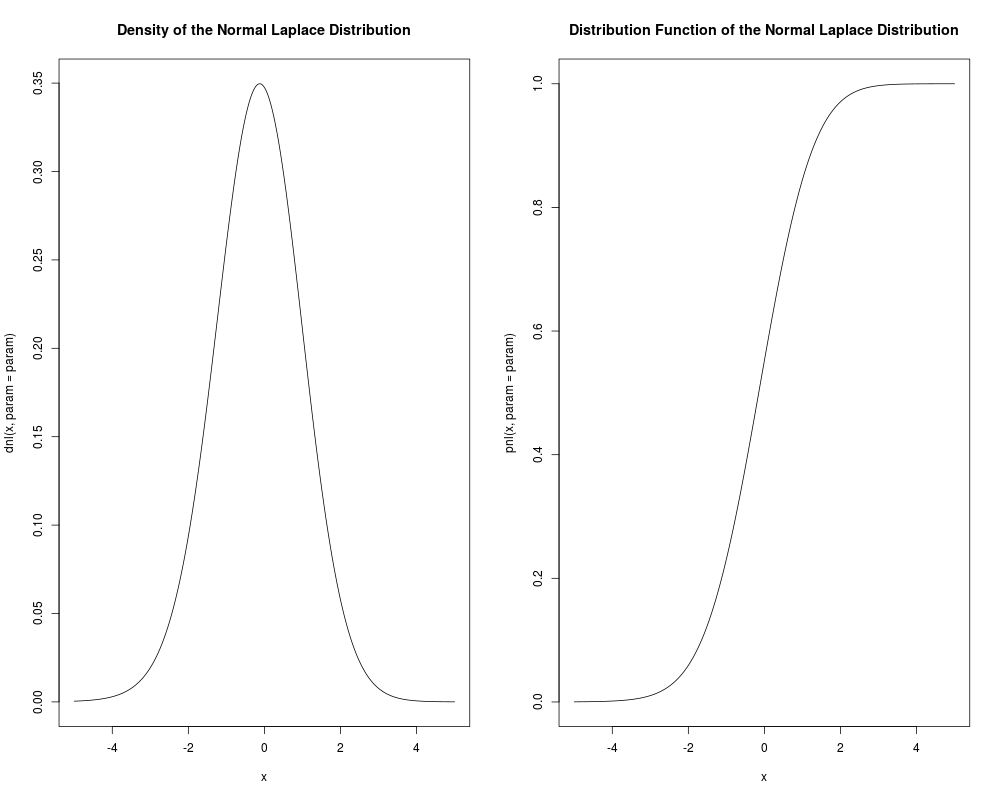
param <- c(0,1,3,2)
par(mfrow = c(1,2))


## Curves of density and distribution
curve(dnl(x, param = param), -5, 5, n = 1000)
title("Density of the Normal Laplace Distribution")
curve(pnl(x, param = param), -5, 5, n = 1000)
title("Distribution Function of the Normal Laplace Distribution")


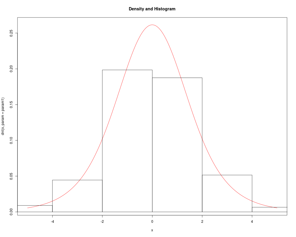
## Example of density and random numbers
 par(mfrow = c(1,1))
 param1  <-  c(0,1,1,1)
 data1  <-  rnl(1000, param = param1)
 curve(dnl(x, param = param1),
       from = -5, to = 5, n = 1000, col = 2)
 hist(data1, freq = FALSE, add = TRUE)
 title("Density and Histogram")

Results

R version 3.3.1 (2016-06-21) -- "Bug in Your Hair"
Copyright (C) 2016 The R Foundation for Statistical Computing
Platform: x86_64-pc-linux-gnu (64-bit)

R is free software and comes with ABSOLUTELY NO WARRANTY.
You are welcome to redistribute it under certain conditions.
Type 'license()' or 'licence()' for distribution details.

R is a collaborative project with many contributors.
Type 'contributors()' for more information and
'citation()' on how to cite R or R packages in publications.

Type 'demo()' for some demos, 'help()' for on-line help, or
'help.start()' for an HTML browser interface to help.
Type 'q()' to quit R.

> library(NormalLaplace)
Loading required package: DistributionUtils
Loading required package: RUnit
Loading required package: GeneralizedHyperbolic
> png(filename="/home/ddbj/snapshot/RGM3/R_CC/result/NormalLaplace/NormalLaplace.Rd_%03d_medium.png", width=480, height=480)
> ### Name: NormalLaplaceDistribution
> ### Title: Normal Laplace Distribution
> ### Aliases: NormalLaplaceDistribution dnl pnl qnl rnl
> ### Keywords: distribution
> 
> ### ** Examples
> 
> param <- c(0,1,3,2)
> par(mfrow = c(1,2))
> 
> 
> ## Curves of density and distribution
> curve(dnl(x, param = param), -5, 5, n = 1000)
> title("Density of the Normal Laplace Distribution")
> curve(pnl(x, param = param), -5, 5, n = 1000)
> title("Distribution Function of the Normal Laplace Distribution")
> 
> 
> ## Example of density and random numbers
>  par(mfrow = c(1,1))
>  param1  <-  c(0,1,1,1)
>  data1  <-  rnl(1000, param = param1)
>  curve(dnl(x, param = param1),
+        from = -5, to = 5, n = 1000, col = 2)
>  hist(data1, freq = FALSE, add = TRUE)
>  title("Density and Histogram")
> 
> 
> 
> 
> 
> 
> 
> dev.off()
null device 
          1 
>