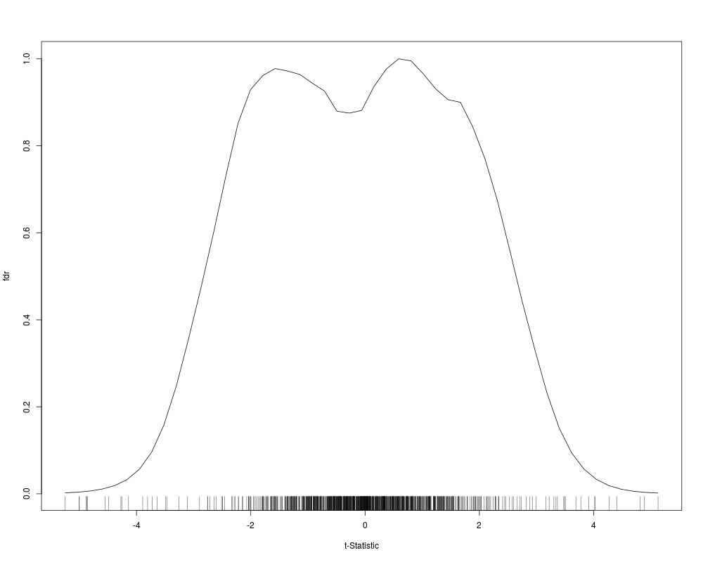
Plot univariate local false discovery output

Description

A plotting function for fdr1d.

Usage

plot.fdr1d.result(x, add = FALSE, grid = FALSE, rug = TRUE, 
                  xlab = "t-Statistic", ylab = "fdr", lcol = "black", ...)

Arguments

Author(s)

A Ploner

See Also

fdr1d

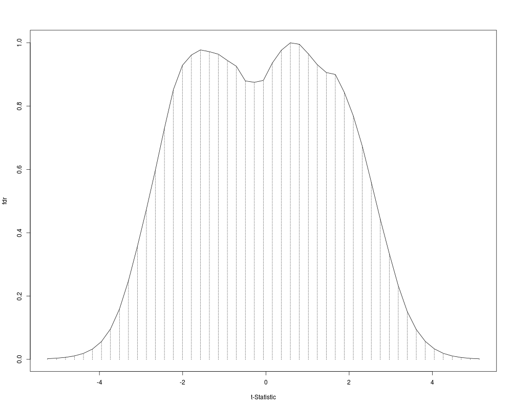
Examples

example(fdr1d)
plot(res1d, grid=TRUE, rug=FALSE)

Results

R version 3.3.1 (2016-06-21) -- "Bug in Your Hair"
Copyright (C) 2016 The R Foundation for Statistical Computing
Platform: x86_64-pc-linux-gnu (64-bit)

R is free software and comes with ABSOLUTELY NO WARRANTY.
You are welcome to redistribute it under certain conditions.
Type 'license()' or 'licence()' for distribution details.

R is a collaborative project with many contributors.
Type 'contributors()' for more information and
'citation()' on how to cite R or R packages in publications.

Type 'demo()' for some demos, 'help()' for on-line help, or
'help.start()' for an HTML browser interface to help.
Type 'q()' to quit R.

> library(OCplus)
Loading required package: akima
> png(filename="/home/ddbj/snapshot/RGM3/R_BC/result/OCplus/plot.fdr1d.result.Rd_%03d_medium.png", width=480, height=480)
> ### Name: plot.fdr1d.result
> ### Title: Plot univariate local false discovery output
> ### Aliases: plot.fdr1d.result
> ### Keywords: hplot aplot
> 
> ### ** Examples
> 
> example(fdr1d)

fdr1d> # We simulate a small example with 5 percent regulated genes and
fdr1d> # a rather large effect size
fdr1d> set.seed(2000)

fdr1d> xdat = matrix(rnorm(50000), nrow=1000)

fdr1d> xdat[1:25, 1:25] = xdat[1:25, 1:25] - 1

fdr1d> xdat[26:50, 1:25] = xdat[26:50, 1:25] + 1

fdr1d> grp = rep(c("Sample A","Sample B"), c(25,25))

fdr1d> # A default run
fdr1d> res1d = fdr1d(xdat, grp)
Starting permutations...
	 1 
	 2 
	 3 
	 4 
	 5 
	 6 
	 7 
	 8 
	 9 
	 10 
	 11 
	 12 
	 13 
	 14 
	 15 
	 16 
	 17 
	 18 
	 19 
	 20 
	 21 
	 22 
	 23 
	 24 
	 25 
	 26 
	 27 
	 28 
	 29 
	 30 
	 31 
	 32 
	 33 
	 34 
	 35 
	 36 
	 37 
	 38 
	 39 
	 40 
	 41 
	 42 
	 43 
	 44 
	 45 
	 46 
	 47 
	 48 
	 49 
	 50 
	 51 
	 52 
	 53 
	 54 
	 55 
	 56 
	 57 
	 58 
	 59 
	 60 
	 61 
	 62 
	 63 
	 64 
	 65 
	 66 
	 67 
	 68 
	 69 
	 70 
	 71 
	 72 
	 73 
	 74 
	 75 
	 76 
	 77 
	 78 
	 79 
	 80 
	 81 
	 82 
	 83 
	 84 
	 85 
	 86 
	 87 
	 88 
	 89 
	 90 
	 91 
	 92 
	 93 
	 94 
	 95 
	 96 
	 97 
	 98 
	 99 
	 100 
Smoothing f
Smoothing f0

fdr1d> res1d[1:20,]
       tstat   fdr.local
1  -3.113975 0.343518819
2  -4.868530 0.005661948
3  -4.487968 0.014988680
4  -3.891546 0.067078413
5  -2.323968 0.794599504
6  -2.491116 0.697740540
7  -2.896670 0.460201903
8  -4.254195 0.026995885
9  -3.490224 0.170529676
10 -3.465717 0.180666869
11 -2.642704 0.605687562
12 -1.532776 0.976587492
13 -3.805811 0.082774181
14 -4.138912 0.035586709
15 -4.999346 0.004067203
16 -3.724595 0.098722065
17 -4.853666 0.005843152
18 -2.607185 0.627256785
19 -3.639713 0.123482696
20 -4.881803 0.005500135

fdr1d> # Looking at the results
fdr1d> summary(res1d)
$Statistic
     Min.   1st Qu.    Median      Mean   3rd Qu.      Max. 
-5.247000 -0.647800 -0.003438  0.015690  0.736200  5.126000 

$fdr
         fdr
statistic (0,0.05] (0.05,0.1] (0.1,0.2] (0.2,1] (1,Inf]
     t<0         8          2         6     480       0
     t>=0       11          3         3     487       0

$p0
$p0$Value
[1] 0.8879223

$p0$Estimated
[1] TRUE



fdr1d> plot(res1d)

fdr1d> res1d[res1d$fdr<0.05, ]
        tstat   fdr.local
2   -4.868530 0.005661948
3   -4.487968 0.014988680
8   -4.254195 0.026995885
14  -4.138912 0.035586709
15  -4.999346 0.004067203
17  -4.853666 0.005843152
20  -4.881803 0.005500135
21  -4.273400 0.025780390
22  -5.247257 0.002150341
23  -4.550108 0.012704082
24  -5.002789 0.004025231
28   4.027545 0.035205867
30   4.274270 0.018487088
32   3.913886 0.047579527
37   4.810875 0.004376113
38   5.125711 0.001711363
39   4.883544 0.003480536
41   4.404355 0.013438726
522  4.017566 0.036292167

fdr1d> # Averaging estimates the global FDR for a set of genes
fdr1d> ndx = abs(res1d$tstat) > 3

fdr1d> mean(res1d$fdr[ndx])
[1] 0.08513626

fdr1d> # Extra information
fdr1d> class(res1d)
[1] "fdr1d.result" "fdr.result"   "data.frame"  

fdr1d> attr(res1d,"param")
$p0
[1] 0.8879223

$p0.est
[1] TRUE

$fdr
 [1] 0.002150341 0.003679441 0.006313912 0.010908497 0.018853690 0.032531021
 [7] 0.056260686 0.095823210 0.158862377 0.248254978 0.357555584 0.474579801
[13] 0.598819090 0.730049134 0.852474483 0.928910674 0.961551113 0.977649650
[19] 0.972012961 0.963954436 0.944227575 0.925816181 0.879585482 0.875265249
[25] 0.881280571 0.936401140 0.976673462 1.000000000 0.995431165 0.965258323
[31] 0.930756968 0.906137071 0.900032160 0.843371879 0.769103282 0.673382987
[37] 0.559230197 0.442600785 0.334090209 0.232379026 0.150794383 0.094266063
[43] 0.056810882 0.033284476 0.018990523 0.010603980 0.005822593 0.003159320
[49] 0.001711363

$xbreaks
 [1] -5.35530881 -5.13920530 -4.92310180 -4.70699829 -4.49089478 -4.27479127
 [7] -4.05868776 -3.84258426 -3.62648075 -3.41037724 -3.19427373 -2.97817022
[13] -2.76206672 -2.54596321 -2.32985970 -2.11375619 -1.89765268 -1.68154918
[19] -1.46544567 -1.24934216 -1.03323865 -0.81713514 -0.60103164 -0.38492813
[25] -0.16882462  0.04727889  0.26338240  0.47948590  0.69558941  0.91169292
[31]  1.12779643  1.34389994  1.56000344  1.77610695  1.99221046  2.20831397
[37]  2.42441748  2.64052098  2.85662449  3.07272800  3.28883151  3.50493502
[43]  3.72103852  3.93714203  4.15324554  4.36934905  4.58545256  4.80155606
[49]  5.01765957  5.23376308

> plot(res1d, grid=TRUE, rug=FALSE)
> 
> 
> 
> 
> 
> dev.off()
null device 
          1 
>