R Graphical Manual

Browse All

Last data update: 2014.03.03

R: FDR as a function of sample size

samplesize

R Documentation

FDR as a function of sample size

Description

This function tabulates the false discovery rate (FDR) for selecting differentially expressed genes as a function of sample size and cutoff level. Additionally, the same information can be displayed through an attractive plot.

Usage

samplesize(n = seq(5, 50, by = 5), p0 = 0.99, sigma = 1, D, F0, F1, 
           paired = FALSE, crit, crit.style = c("top percentage", "cutoff"),
		   plot =TRUE, local.show=FALSE, nplot = 100, ylim = c(0, 1), main,
		   legend.show = FALSE, grid.show = FALSE, ...)

Arguments

`n`	sample size (as subjects per group)
`p0`	the proportion of non-differentially expressed genes
`sigma`	the standard deviation for the log expression values
`D`	assumed average log fold change (in units of `sigma`), by default 1; this is a shortcut for specifying a simple symmetrical alternative hypothesis through `F1`.
`F0`	the distribution of the log2 expression values under the null hypothesis; by default, this is normal with mean zero and standard deviation `sigma`, but mixtures of normals can be specified, see Details and Examples.
`F1`	the distribution of the log2 expression values under the alternative hypothesis; by default, this is an equal mixture of two normals with means `D` and -`D` and standard deviation `sigma`; mixture of normals are again possible, see Details and Examples.
`paired`	logical value indicating whether this is the independent sample case (default) or the paired sample case.
`crit`	a vector of cutoff values for selecting differentially expressed genes; the interpretation depends on `crit.style`.
`crit.style`	indicates how differentially expressed genes are selected: either by a fixed cutoff level for the absolute value of the t-statistic or as a fixed percentage of the absolute largest t-statistics.
`plot`	logical value indicating whether to do the plotting business
`local.show`	logical value indicating whether to show local or global false discovery rate (default: global).
`nplot`	number of points that are evaluated for the curves
`ylim`	the usual limits on the vertical axis
`main`	the main title of the plot
`legend.show`	logical value indicating whether to show a legend for the types of gene selection in the plot
`grid.show`	logical value indicating whether to draw grid lines showing the sample sizes `n` to be tabulated in the plot
`...`	the usual graphical parameters, passed to `plot`

Details

This function plots the FDR as a function of the sample size when comparing the expression of multiple genes between two groups of subjects. This is based on a model assuming that a proportion p0 of genes is not differentially expressed (regulated) between groups, and that 1-p0 genes are. The logarithmized gene expression values of regulated and non regulated genes are assumed to be generated by mixtures of normal distributions; these mixtures can be specified through the parameters F0, F1 or D, and sigma; please see TOC for details on the model and the specification of the mixtures. By default, the null distribution of the log expression values is a normal centered on zero, and the alternative an equal mixture of normals centered at +D and -D.

The list of nominally differentially expressed genes can be selected in two ways:

all genes with absolute t-statistic larger than the specified critical cutoff values (cutoff),
all genes that represent the specified critical top percentage of the absolutely largest t-statistics (top percentage).

Multiple critical values correspond to multiple curves, each labeled by the critical value, but only one value can be specified for the proportion of non-regulated genes p0 and the standard deviation sigma.

Value

A matrix with rows corresponding to elements of n and columns corresponding to the specified critical values is returned. The matrix has the attribute param that contains the specified arguments, see Examples.

Note

Both the curve labels and the legend may be squashed if the plotting device is too small. Increasing the size of the device and re-plotting should improve readability.

Author(s)

Y. Pawitan and A. Ploner

References

Pawitan Y, Michiels S, Koscielny S, Gusnanto A, Ploner A (2005) False Discovery Rate, Sensitivity and Sample Size for Microarray Studies. Bioinformatics, 21, 3017-3024.

Jung SH (2005) Sample size for FDR-control in microarray data analysis. Bioinformatics, 21, 3097-104.

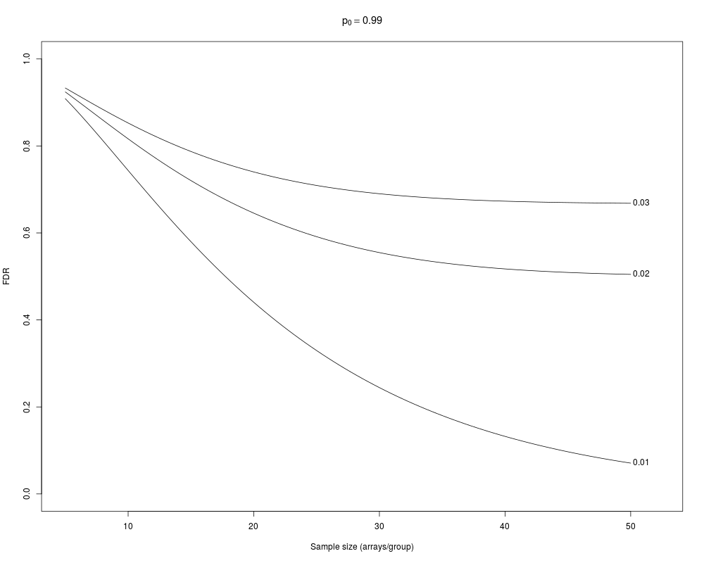
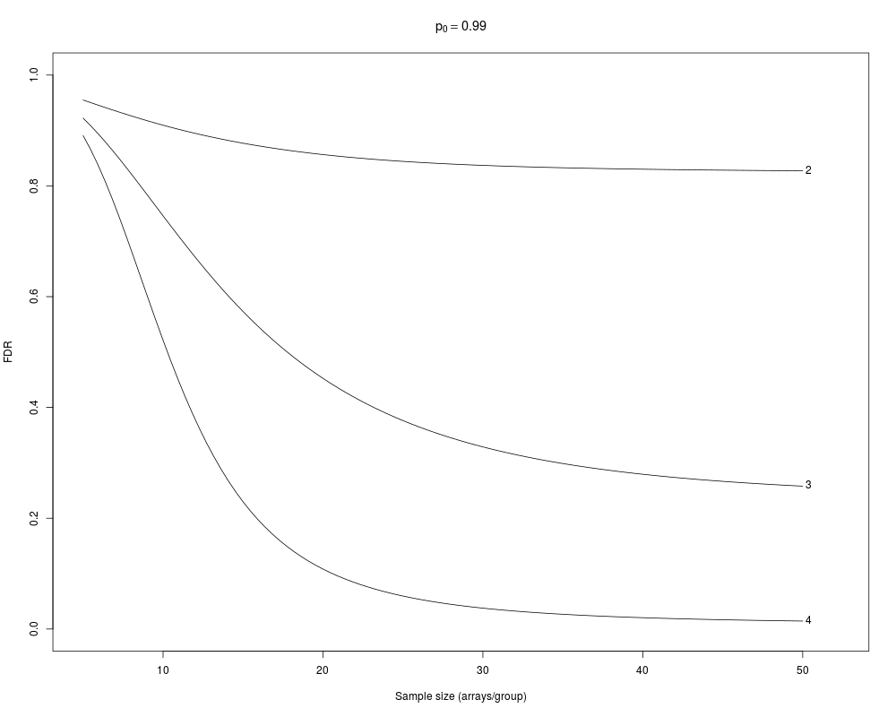
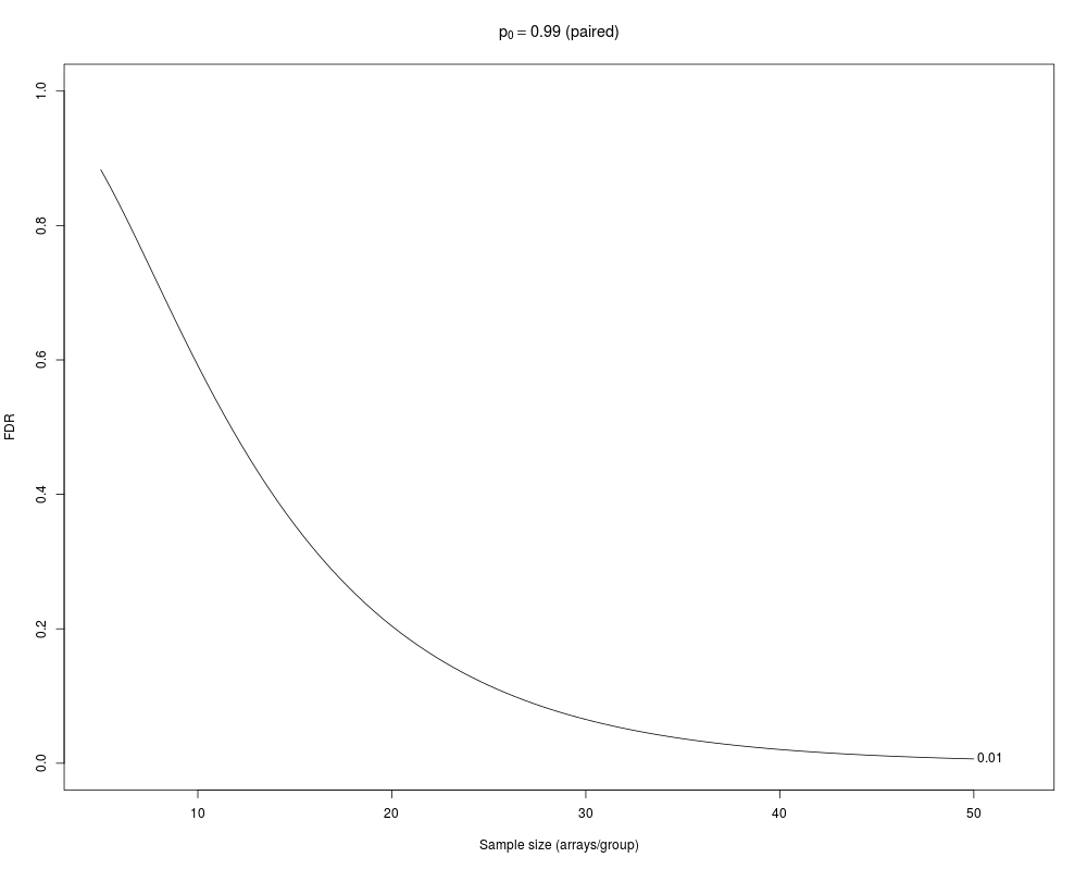
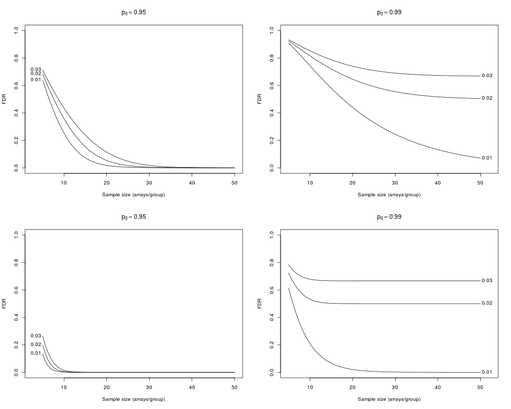
Examples

# Default assumes a proportion of 0.01 regulated genes equally split
# between two-fold up- and down-regulated
# We select the top 1, 2, 3 percent absolute largest t-statistics
samplesize(crit=c(0.03,0.02, 0.01))

# Same model, but using a hard cutoff for the t-statistics
samplesize(crit=2:4, crit.style="cutoff")

# Paired test of the same size has slightly better FDR (as expected)
samplesize(paired=TRUE)

# Compare the effect of p0 and effect size
par(mfrow=c(2,2))
samplesize(crit=c(0.03,0.02, 0.01), p0=0.95, D=1)
samplesize(crit=c(0.03,0.02, 0.01), p0=0.99, D=1)
samplesize(crit=c(0.03,0.02, 0.01), p0=0.95, D=2)
samplesize(crit=c(0.03,0.02, 0.01), p0=0.99, D=2)

# An asymmetric alternative distribution: 20 percent of the regulated genes 
# are expected to be (at least) four-fold up regulated
# NB, no graphical output
ret = samplesize(F1=list(D=c(-1,1,2), p=c(2,2,1)), p0=0.95, crit=0.05, plot=FALSE)
ret
# Look at the parameters
attr(ret, "param")

# A wide null distribution that allows to disregard genes with small effect
# Here: |log2 fold change| < 0.25, i.e. fold change of less than 19 percent
samplesize(F0=list(D=c(-0.25,0,0.25)), grid=TRUE)

# This is close to Example 3 in Jung's paper (see References):
# p0=0.99 and sensitivity=0.6, so we want a rejection rate of 
# around 0.006 from the top list.
# Here we require around 40 arrays/group, compared to 
# around 37 in Jung's paper, most likely because we use 
# the t-distribution instead of normal. Jung's alternative 
# is only one-sided, so the exact correspondence is
# 
samplesize(p0=0.99,crit.style="top", crit=0.006, F1=list(D=1, p=1), grid=TRUE) 
abline(h=0.01)

#The result is very close to the symmetric alternatives: 
samplesize(p0=0.99,crit=0.006, D=1, grid=TRUE, ylim=c(0,0.9))

Results


R version 3.3.1 (2016-06-21) -- "Bug in Your Hair"
Copyright (C) 2016 The R Foundation for Statistical Computing
Platform: x86_64-pc-linux-gnu (64-bit)

R is free software and comes with ABSOLUTELY NO WARRANTY.
You are welcome to redistribute it under certain conditions.
Type 'license()' or 'licence()' for distribution details.

R is a collaborative project with many contributors.
Type 'contributors()' for more information and
'citation()' on how to cite R or R packages in publications.

Type 'demo()' for some demos, 'help()' for on-line help, or
'help.start()' for an HTML browser interface to help.
Type 'q()' to quit R.

> library(OCplus)
Loading required package: akima
> png(filename="/home/ddbj/snapshot/RGM3/R_BC/result/OCplus/samplesize.Rd_%03d_medium.png", width=480, height=480)
> ### Name: samplesize
> ### Title: FDR as a function of sample size
> ### Aliases: samplesize
> ### Keywords: hplot design
> 
> ### ** Examples
> 
> # Default assumes a proportion of 0.01 regulated genes equally split
> # between two-fold up- and down-regulated
> # We select the top 1, 2, 3 percent absolute largest t-statistics
> samplesize(crit=c(0.03,0.02, 0.01))
    FDR_0.03  FDR_0.02   FDR_0.01  fdr_0.03  fdr_0.02  fdr_0.01
5  0.9332083 0.9241507 0.90862674 0.9553806 0.9465999 0.9308308
10 0.8527357 0.8163128 0.74363226 0.9364990 0.9120815 0.8566299
15 0.7872589 0.7203631 0.57984481 0.9367426 0.9006521 0.8007015
20 0.7402120 0.6454597 0.44048579 0.9472731 0.9055975 0.7586710
25 0.7091729 0.5914074 0.32960863 0.9612547 0.9205747 0.7263381
30 0.6901142 0.5548012 0.24436951 0.9742294 0.9396772 0.7007974
35 0.6790658 0.5314253 0.18012346 0.9841715 0.9581346 0.6801693
40 0.6729944 0.5173024 0.13226434 0.9908775 0.9731218 0.6631697
45 0.6698018 0.5091891 0.09687714 0.9950014 0.9838281 0.6489225
50 0.6681810 0.5047281 0.07083547 0.9973696 0.9907684 0.6367946
There were 50 or more warnings (use warnings() to see the first 50)
> 
> # Same model, but using a hard cutoff for the t-statistics
> samplesize(crit=2:4, crit.style="cutoff")
       FDR_2     FDR_3      FDR_4     fdr_2     fdr_3     fdr_4
5  0.9549312 0.9221888 0.89078815 0.9748323 0.9446546 0.9117790
10 0.9094975 0.7458752 0.52126360 0.9693400 0.8584665 0.6397336
15 0.8769959 0.5731654 0.22971236 0.9741541 0.7950745 0.3799792
20 0.8564746 0.4524831 0.10818649 0.9818348 0.7699947 0.2381503
25 0.8441933 0.3762622 0.05955185 0.9886188 0.7767293 0.1703211
30 0.8369742 0.3287560 0.03769602 0.9934250 0.8043933 0.1387938
35 0.8326899 0.2987451 0.02662720 0.9964259 0.8424982 0.1263607
40 0.8300566 0.2793891 0.02045304 0.9981472 0.8822997 0.1259723
45 0.8283449 0.2665992 0.01674373 0.9990756 0.9177308 0.1351638
50 0.8271549 0.2579029 0.01438464 0.9995531 0.9457889 0.1538027
There were 50 or more warnings (use warnings() to see the first 50)
> 
> # Paired test of the same size has slightly better FDR (as expected)
> samplesize(paired=TRUE)
      FDR_0.01  fdr_0.01
5  0.882939594 0.9027874
10 0.591675057 0.7682531
15 0.354329893 0.6907511
20 0.204095745 0.6434303
25 0.115691714 0.6117082
30 0.065112671 0.5889743
35 0.036524672 0.5718406
40 0.020458850 0.5584287
45 0.011457176 0.5477126
50 0.006416521 0.5388778
There were 50 or more warnings (use warnings() to see the first 50)
> 
> # Compare the effect of p0 and effect size
> par(mfrow=c(2,2))
> samplesize(crit=c(0.03,0.02, 0.01), p0=0.95, D=1)
       FDR_0.03     FDR_0.02     FDR_0.01    fdr_0.03     fdr_0.02     fdr_0.01
5  0.7128707717 6.836793e-01 6.383069e-01 0.786962313 0.7534288017 0.6993141173
10 0.4347044692 3.580158e-01 2.525235e-01 0.634850496 0.5347284898 0.3799927428
15 0.2382994087 1.533038e-01 7.292893e-02 0.488428152 0.3229719130 0.1467379021
20 0.1149068790 5.405150e-02 1.793485e-02 0.331689658 0.1506324924 0.0430765448
25 0.0480418615 1.673463e-02 4.272366e-03 0.185044124 0.0557974503 0.0114247637
30 0.0178095217 4.914207e-03 1.033032e-03 0.083853426 0.0183104756 0.0029846590
35 0.0061463497 1.427652e-03 2.555826e-04 0.032868276 0.0057511196 0.0007864970
40 0.0020559909 4.163564e-04 6.458336e-05 0.011973630 0.0017849333 0.0002098690
45 0.0006803129 1.223274e-04 1.661407e-05 0.004225733 0.0005532039 0.0000566670
50 0.0002245366 3.620509e-05 4.338653e-06 0.001471592 0.0001717043 0.0000154595
There were 50 or more warnings (use warnings() to see the first 50)
> samplesize(crit=c(0.03,0.02, 0.01), p0=0.99, D=1)
    FDR_0.03  FDR_0.02   FDR_0.01  fdr_0.03  fdr_0.02  fdr_0.01
5  0.9332083 0.9241507 0.90862674 0.9553806 0.9465999 0.9308308
10 0.8527357 0.8163128 0.74363226 0.9364990 0.9120815 0.8566299
15 0.7872589 0.7203631 0.57984481 0.9367426 0.9006521 0.8007015
20 0.7402120 0.6454597 0.44048579 0.9472731 0.9055975 0.7586710
25 0.7091729 0.5914074 0.32960863 0.9612547 0.9205747 0.7263381
30 0.6901142 0.5548012 0.24436951 0.9742294 0.9396772 0.7007974
35 0.6790658 0.5314253 0.18012346 0.9841715 0.9581346 0.6801693
40 0.6729944 0.5173024 0.13226434 0.9908775 0.9731218 0.6631697
45 0.6698018 0.5091891 0.09687714 0.9950014 0.9838281 0.6489225
50 0.6681810 0.5047281 0.07083547 0.9973696 0.9907684 0.6367946
There were 50 or more warnings (use warnings() to see the first 50)
> samplesize(crit=c(0.03,0.02, 0.01), p0=0.95, D=2)
       FDR_0.03     FDR_0.02     FDR_0.01     fdr_0.03     fdr_0.02
5  2.640229e-01 2.002557e-01 1.348339e-01 4.524080e-01 3.292586e-01
10 1.505733e-02 5.704655e-03 1.928410e-03 5.925395e-02 1.696187e-02
15 4.802034e-04 1.278324e-04 2.970820e-05 2.458784e-03 4.666986e-04
20 1.490721e-05 3.052755e-06 5.232062e-07 8.836656e-05 1.277928e-05
25 4.687633e-07 7.630549e-08 1.000594e-08 3.107771e-06 3.553025e-07
30 1.486560e-08 1.966194e-09 2.024204e-10 1.079948e-07 9.991079e-09
35 4.739875e-10 5.178623e-11 4.260983e-12 3.720639e-09 2.833981e-10
40 1.515972e-11 1.392220e-12 8.437558e-14 1.272886e-10 8.092700e-12
45 4.886827e-13 4.218784e-14 0.000000e+00 4.330340e-12 2.323996e-13
50 1.406285e-14 0.000000e+00 0.000000e+00 1.466237e-13 6.703617e-15
       fdr_0.01
5  2.020542e-01
10 4.361612e-03
15 8.049273e-05
20 1.611341e-06
25 3.407346e-08
30 7.489149e-10
35 1.694392e-11
40 3.921771e-13
45 9.246487e-15
50 2.214097e-16
There were 50 or more warnings (use warnings() to see the first 50)
> samplesize(crit=c(0.03,0.02, 0.01), p0=0.99, D=2)
    FDR_0.03  FDR_0.02     FDR_0.01  fdr_0.03  fdr_0.02  fdr_0.01
5  0.7829529 0.7234879 6.136961e-01 0.9216066 0.8769829 0.7724204
10 0.6783697 0.5330225 2.097715e-01 0.9818472 0.9477440 0.6427297
15 0.6673258 0.5025297 6.661388e-02 0.9985460 0.9937154 0.5880059
20 0.6666926 0.5001183 2.087776e-02 0.9999260 0.9995864 0.5575539
25 0.6666683 0.4999889 6.537649e-03 0.9999971 0.9999799 0.5381180
30 0.6666672 0.4999821 2.051126e-03 0.9999999 0.9999992 0.5244981
35 0.6666667 0.4999812 6.455354e-04 1.0000000 1.0000000 0.5145312
40 0.6666667 0.4999807 2.037386e-04 1.0000000 1.0000000 0.5068137
45 0.6666667 0.4999804 6.448653e-05 1.0000000 1.0000000 0.5007262
50 0.6666667 0.4999803 2.046001e-05 1.0000000 1.0000000 0.4957181
There were 50 or more warnings (use warnings() to see the first 50)
> 
> # An asymmetric alternative distribution: 20 percent of the regulated genes 
> # are expected to be (at least) four-fold up regulated
> # NB, no graphical output
> ret = samplesize(F1=list(D=c(-1,1,2), p=c(2,2,1)), p0=0.95, crit=0.05, plot=FALSE)
There were 50 or more warnings (use warnings() to see the first 50)
> ret
     FDR_0.05  fdr_0.05
5  0.66971585 0.8127709
10 0.46108555 0.7623678
15 0.33037347 0.7198752
20 0.23738850 0.6868708
25 0.17044536 0.6619586
30 0.12237610 0.6426787
35 0.08790549 0.6272889
40 0.06319821 0.6147207
45 0.04547885 0.6042473
50 0.03275884 0.5953623
> # Look at the parameters
> attr(ret, "param")
$p0
[1] 0.95

$sigma
[1] 1

$F0
$F0$D
[1] 0

$F0$p
[1] 1


$F1
$F1$D
[1] -1  1  2

$F1$p
[1] 0.4 0.4 0.2


$paired
[1] FALSE

$crit.style
[1] "top percentage"

> 
> # A wide null distribution that allows to disregard genes with small effect
> # Here: |log2 fold change| < 0.25, i.e. fold change of less than 19 percent
> samplesize(F0=list(D=c(-0.25,0,0.25)), grid=TRUE)
    FDR_0.01  fdr_0.01
5  0.9230888 0.9391629
10 0.8030289 0.8776216
15 0.6846516 0.8293377
20 0.5781154 0.7913151
25 0.4856788 0.7608630
30 0.4068610 0.7360090
35 0.3403032 0.7154034
40 0.2843634 0.6980323
45 0.2375012 0.6832077
50 0.1983093 0.6704032
There were 50 or more warnings (use warnings() to see the first 50)
> 
> # This is close to Example 3 in Jung's paper (see References):
> # p0=0.99 and sensitivity=0.6, so we want a rejection rate of 
> # around 0.006 from the top list.
> # Here we require around 40 arrays/group, compared to 
> # around 37 in Jung's paper, most likely because we use 
> # the t-distribution instead of normal. Jung's alternative 
> # is only one-sided, so the exact correspondence is
> # 
> samplesize(p0=0.99,crit.style="top", crit=0.006, F1=list(D=1, p=1), grid=TRUE) 
     FDR_0.006   fdr_0.006
5  0.897438109 0.918985085
10 0.683641755 0.804726142
15 0.464404611 0.691126071
20 0.283170460 0.567306126
25 0.152361220 0.423040156
30 0.070702112 0.266811701
35 0.028330270 0.135298381
40 0.010209456 0.056720440
45 0.003483354 0.021259587
50 0.001162771 0.007573181
There were 50 or more warnings (use warnings() to see the first 50)
> abline(h=0.01)
> 
> #The result is very close to the symmetric alternatives: 
> samplesize(p0=0.99,crit=0.006, D=1, grid=TRUE, ylim=c(0,0.9))
     FDR_0.006   fdr_0.006
5  0.897438109 0.918985085
10 0.683641755 0.804726142
15 0.464404611 0.691126071
20 0.283170460 0.567306126
25 0.152361220 0.423040156
30 0.070702112 0.266811701
35 0.028330270 0.135298381
40 0.010209456 0.056720440
45 0.003483354 0.021259587
50 0.001162771 0.007573181
There were 50 or more warnings (use warnings() to see the first 50)
> 
> 
> 
> 
> 
> 
> dev.off()
null device 
          1 
>