Between-array scaling

Description

This function performs an between-array scaling

Usage

bas(obj,mode="var")

Arguments

Details

The function bsv adjust the scale of logged ratios (M=(log2(Ch2)-log2(Ch1))) between the different arrays stored in obj.

Following schemes (mode) are implemented:

• mode="var": Logged ratios M are scaled to show the same (within-array) variance for all arrays in the batch stored in obj. The variance is calculated using var.

• mode="mad": The same procedure as for mode="var" is applied using, however, median absolute deviation (mad) as robust estimate for withing-array variance.

• mode="qq": The quantile scaling is using the same procedure as the quantile normalisation described by Bolstad et al. (2003). In brief: Given X is the matrix with logged ratios (column corresponding to arrays, rows to genes)

  1. Sort each column of X (independently) producing Xs,

  2. Replace values in each row of Xs by the mean value of the row producing Xsm,

  3. Rearrange the ordering for each column of matrix Xsm, so that it has the columns have same ordering as for the original matrix X.

  The last step yields the scaled logged ratios M.

Note

Between-array scaling should only be performed if it can be assumed that the different arrays have a similar distribution of logged ratios. This has to be check on a case-by-case basis. Caution should be taken in the interpretation of results for arrays hybridised with biologically divergent samples, if between-array scaling is applied.

Author(s)

Matthias E. Futschik (http://itb.biologie.hu-berlin.de/~futschik)

References

Bolstad et al., A comparison of normalization methods for high density oligonucleotide array data based on variance and bias, Bioinformatics, 19: 185-193, 2003

See Also

marrayNorm,var,mad

Examples

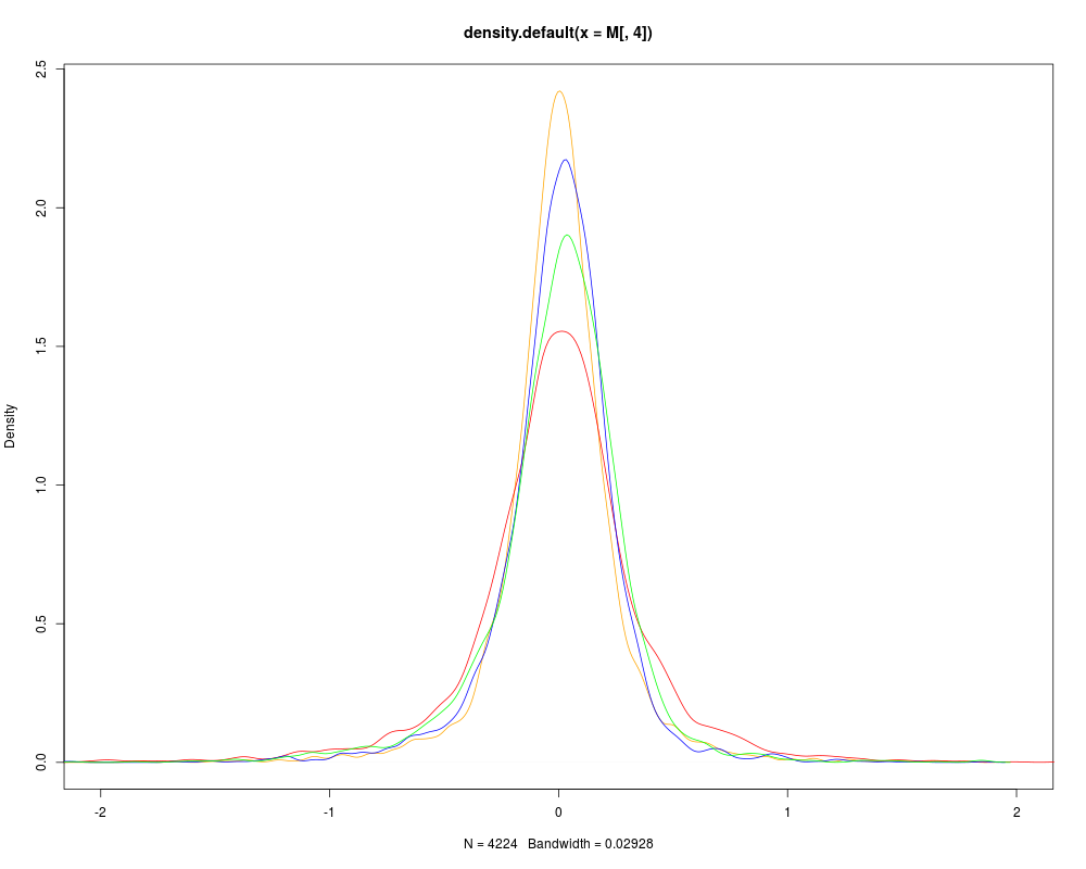
# DISTRIBUTION OF M BEFORE SCALING
data(sw.olin)

col <- c("red","blue","green","orange")
M <- maM(sw.olin)

plot(density(M[,4]),col=col[4],xlim=c(-2,2))
for (i in 1:3){
  lines(density(M[,i]),col=col[i])
}


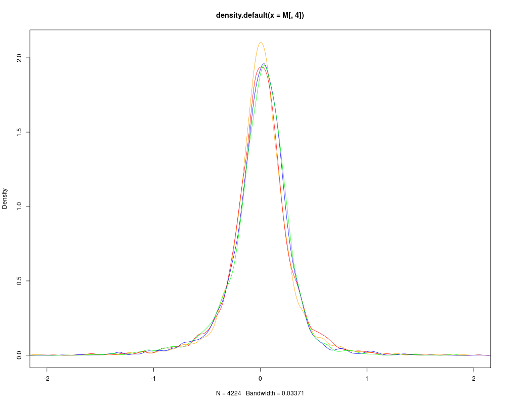
# SCALING AND VISUALISATION  
sw.olin.s <- bas(sw.olin,mode="var")
  
M <- maM(sw.olin.s)

plot(density(M[,4]),col=col[4],xlim=c(-2,2))
for (i in 1:3){
  lines(density(M[,i]),col=col[i])
}

Results

R version 3.3.1 (2016-06-21) -- "Bug in Your Hair"
Copyright (C) 2016 The R Foundation for Statistical Computing
Platform: x86_64-pc-linux-gnu (64-bit)

R is free software and comes with ABSOLUTELY NO WARRANTY.
You are welcome to redistribute it under certain conditions.
Type 'license()' or 'licence()' for distribution details.

R is a collaborative project with many contributors.
Type 'contributors()' for more information and
'citation()' on how to cite R or R packages in publications.

Type 'demo()' for some demos, 'help()' for on-line help, or
'help.start()' for an HTML browser interface to help.
Type 'q()' to quit R.

> library(OLIN)
Loading required package: locfit
locfit 1.5-9.1 	 2013-03-22
Loading required package: marray
Loading required package: limma
> png(filename="/home/ddbj/snapshot/RGM3/R_BC/result/OLIN/bas.Rd_%03d_medium.png", width=480, height=480)
> ### Name: bas
> ### Title: Between-array scaling
> ### Aliases: bas
> ### Keywords: utilities
> 
> ### ** Examples
> 
> 
> 
> # DISTRIBUTION OF M BEFORE SCALING
> data(sw.olin)
> 
> col <- c("red","blue","green","orange")
> M <- maM(sw.olin)
> 
> plot(density(M[,4]),col=col[4],xlim=c(-2,2))
> for (i in 1:3){
+   lines(density(M[,i]),col=col[i])
+ }
> 
> 
> # SCALING AND VISUALISATION  
> sw.olin.s <- bas(sw.olin,mode="var")
>   
> M <- maM(sw.olin.s)
> 
> plot(density(M[,4]),col=col[4],xlim=c(-2,2))
> for (i in 1:3){
+   lines(density(M[,i]),col=col[i])
+ }
> 
> 
> 
> 
> 
> 
> dev.off()
null device 
          1 
>