R Graphical Manual

Browse All

Last data update: 2014.03.03

R: Local intensity-dependent normalisation of two-colour...

lin	R Documentation

Local intensity-dependent normalisation of two-colour microarrays

Description

This functions performs local intensity-dependent normalisation (LIN)

Usage

lin(object,X=NA,Y=NA,alpha=0.3,iter=2,scale=TRUE,weights=NA,bg.corr="subtract",...)

Arguments

`object`	object of class “marrayRaw”
`X`	matrix with x-coordinates of spots. If X=NA, columns on array are used as proxies for the location in x-direction
`Y`	matrix with y-coordinates of spots. If Y=NA, rows on array are used as proxies for the location in y-direction
`alpha`	smooting parameter for local regression
`iter`	number of iterations in the LIN procedure
`scale`	scale parameter for smooting in Y-direction of the array in respect to smoothing in X-direcction. If `scale=TRUE`, standard deviations are used.
`weights`	matrix of weights for local regression. Rows correspond to the spotted probe sequences, columns to arrays in the batch. These may be derived from the matrix of spot quality weights as defined for “maRaw” objects.
`bg.corr`	backcorrection method (for “marrayRaw” objects) : “none” or “subtract”(default).
`...`	Further arguments for `locfit` function.

Details

LIN is based on the same normalisation scheme as OLIN, but does not incorporate optimisation of model parameters. The function lin can serve for comparison. Alternatively, it can be used to enforce a conservative model fit.

The smoothing parameter alpha controls the neighbourhood size h of local fitting. It specifies the fraction of points that are included in the neighbourhood and, thus, has a value between 0 and 1. Larger alpha values lead to smoother fits.

If the normalisation should be based on set of genes assumed to be not differentially expressed (house-keeping genes), weights can be used for local regression. In this case, all weights should be set to zero except for the house-keeping genes for which weights are set to one. In order to achieve a reliable regression, it is important, however, that there is a sufficient number of house-keeping genes that cover the whole expression range and are spotted accross the whole array.

Value

Object of class “marrayNorm” with normalised logged ratios

Author(s)

Matthias E. Futschik (http://itb.biologie.hu-berlin.de/~futschik)

References

M.Futschik and T.Crompton (2004) Model selection and efficiency testing for normalization of cDNA microarray data, Genome Biology, 5:R60

Examples




# LOADING DATA
  data(sw)
  data(sw.xy)

# LOCAL INTENSITY-DEPENDENT NORMALISATION 
 norm.lin <- lin(sw,X=sw.xy$X,Y=sw.xy$Y)

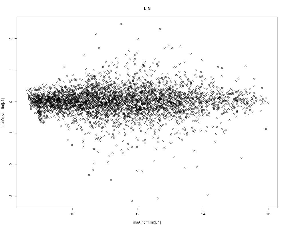
# MA-PLOT OF NORMALISATION RESULTS OF FIRST ARRAY
 plot(maA(norm.lin)[,1],maM(norm.lin)[,1],main="LIN")
 
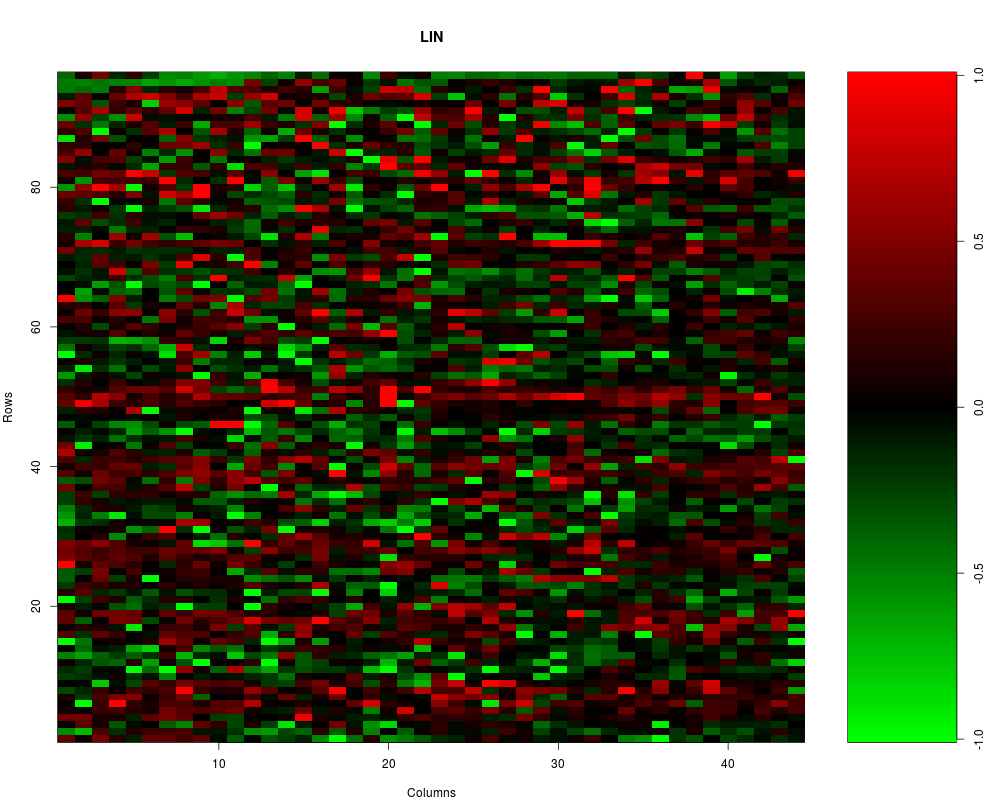
# CORRESPONDING MXY-PLOT
   mxy.plot(maM(norm.lin)[,1],Ngc=maNgc(norm.lin),Ngr=maNgr(norm.lin),
                Nsc=maNsc(norm.lin),Nsr=maNsr(norm.lin),main="LIN")

Results


R version 3.3.1 (2016-06-21) -- "Bug in Your Hair"
Copyright (C) 2016 The R Foundation for Statistical Computing
Platform: x86_64-pc-linux-gnu (64-bit)

R is free software and comes with ABSOLUTELY NO WARRANTY.
You are welcome to redistribute it under certain conditions.
Type 'license()' or 'licence()' for distribution details.

R is a collaborative project with many contributors.
Type 'contributors()' for more information and
'citation()' on how to cite R or R packages in publications.

Type 'demo()' for some demos, 'help()' for on-line help, or
'help.start()' for an HTML browser interface to help.
Type 'q()' to quit R.

> library(OLIN)
Loading required package: locfit
locfit 1.5-9.1 	 2013-03-22
Loading required package: marray
Loading required package: limma
> png(filename="/home/ddbj/snapshot/RGM3/R_BC/result/OLIN/lin.Rd_%03d_medium.png", width=480, height=480)
> ### Name: lin
> ### Title: Local intensity-dependent normalisation of two-colour
> ###   microarrays
> ### Aliases: lin
> ### Keywords: utilities regression
> 
> ### ** Examples
> 
> 
> 
> 
> # LOADING DATA
>   data(sw)
>   data(sw.xy)
> 
> # LOCAL INTENSITY-DEPENDENT NORMALISATION 
>  norm.lin <- lin(sw,X=sw.xy$X,Y=sw.xy$Y)
> 
> # MA-PLOT OF NORMALISATION RESULTS OF FIRST ARRAY
>  plot(maA(norm.lin)[,1],maM(norm.lin)[,1],main="LIN")
>  
> # CORRESPONDING MXY-PLOT
>    mxy.plot(maM(norm.lin)[,1],Ngc=maNgc(norm.lin),Ngr=maNgr(norm.lin),
+                 Nsc=maNsc(norm.lin),Nsr=maNsr(norm.lin),main="LIN")
> 
> 
> 
> 
> 
> 
> 
> dev.off()
null device 
          1 
>