R Graphical Manual

Browse All

Last data update: 2014.03.03

R: Optimised local intensity-dependent normalisation of...

olin	R Documentation

Optimised local intensity-dependent normalisation of two-colour microarrays

Description

This functions performs optimised local intensity-dependent normalisation (OLIN) and optimised scaled intensity-dependent normalisation (OSLIN).

Usage

olin(object,X=NA,Y=NA,alpha=seq(0.1,1,0.1),iter=3,
            scale=c(0.05,0.1,0.5,1,2,10,20),OSLIN=FALSE,weights=NA,
            genepix=FALSE,bg.corr="subtract",...)

Arguments

`object`	object of class “marrayRaw” or “marrayNorm” corresponding to a single array or a batch of arrays.
`X`	matrix with x-coordinates of spots of the arrays in `object`. Each column includes the x-coodinates for the spots of one array. If X=NA, columns on array are used as proxies for the location in x-direction
`Y`	matrix with y-coordinates of spots. Each column includes the y-coodinates for the spots of one array.If Y=NA, rows on array are used as proxies for the location in y-direction
`alpha`	vector of alpha parameters that are tested in the GCV procedure
`iter`	number of iterations in the OLIN procedure
`scale`	vector of scale parameters that are tested in a GCV procedure for spatial regression. This define the amount of smoothing in X-direction with respect to smoothing in Y-direction.
`OSLIN`	If OSLIN=TRUE, subsequent scaling of the range of M accross the array is performed.
`weights`	matrix of (non-negative) weights for local regression (see `locfit`). Rows correspond to the spotted probe sequences, columns to arrays in the batch. If the weight of the corresponding spot equals zero, the spot is not used in the normalisation procedures (except the `genepix` argument is set to `TRUE`.) If the weight matrix include negative values, these will be set to zero. These weight matrix may be derived from the matrix of spot quality weights as defined for “maRaw” objects (`weights=maW(object)`. Weights can be also used if the normalisation should be based on a set of selected genes that are assumed to be not differentially expressed.
`genepix`	If `genepix` is set to `TRUE`, spot weights equal zero or larger are set to one for the local regression whereas negative spot with negative weights are not used for the regression. The argument `genepix` should be set to `TRUE`, if `weights=maW(object)` is set and spot quality weights derived by GenePix are stored in `maW(object)`.
`bg.corr`	backcorrection method (for “marrayRaw” objects) : “none”, “subtract”, “half”, “minimum”, “movingmin”, “edwards” or “normexp”.
`...`	Further arguments for `locfit` function.

Details

OLIN and OSLIN are based on iterative local regression and incorporate optimisation of model parameters. Local regression is performed using LOCFIT, which requires the user to choose a specific smoothing parameter alpha that controls the neighbourhood size h of local fitting. The parameter alpha specifies the fraction of points that are included in the neighbourhood and thus has a value between 0 and 1. Larger alpha values lead to smoother fits. Additionally, the setting of scale parameters controls for distinct amount of smoothing in Y-direction compared to smoothing in X-direction. The parameter scale can be of arbitrary value. The choice of model parameters alpha and scale for local regression is crucial for the efficiency and quality of normalization. To optimize the model parameters, a general cross-validation procedure (GCV) is applied. The arguments alpha and scale define the parameters values which are tested in the GCV. OSLIN comprises the OLIN procedure with a subsequent optimized scaling of the range of logged intensity ratios across the spatial dimensions of the array. Details concerning the background correction methods can be found in the help page for backgroundCorrect2.

Detailed information about OLIN and OSLIN can be found in the package documentation and in the reference stated below. The weights argument specifies the influence of the single spots on the local regression. To exclude spots being used for the local regression (such as control spots), set their corresponding weight to zero. Note that OLIN and OSLIN are based on the assumptions that most genes are not differentially expressed (or up- and down-regulation is balanced) and that genes are randomly spotted across the array. If these assumptions are not valid, local regression can lead to an underestimation of differential expression. OSLIN is especially sensitive to violations of these assumptions. However, this sensitivity can be decreased if the minimal alpha-value is increased. Minimal alpha defines the smallest scale used for local regression. Increasing alpha can reduce the influence of localised artifacts as a larger fraction of data points is included. Alternative normalisation functions such as oin, lin and ino might also be used for a more conservative fit.

If the normalisation should be based on set of genes assumed to be not differentially expressed (house-keeping genes), weights can be used for local regression. In this case, all weights are set to zero except for the house-keeping genes for which weights are set to one. In order to achieve a reliable regression, it is important, however, that there is a sufficient number of house-keeping genes that are distributed over the whole expression range and spotted accross the whole array.

It is also important to note that OLIN/OSLIN is fairly efficient in removing intensity- and spatial-dependent dye bias, so that normalised data will look quite “good” after normalisation independently of the true underlying data quality. Normalisation by local regression assumes smoothness of bias. Therefore, localised artifacts such as scratches, edge effects or bubbles should be avoided. Spots of these areas should be flagged (before normalisation is applied) to ensure data integrity. To stringently detect artifacts, the OLIN functions fdr.int, fdr.spatial, p.int and p.spatial can be used.

Value

Object of class “marrayNorm” with normalised logged ratios

Author(s)

Matthias E. Futschik (http://itb.biologie.hu-berlin.de/~futschik)

References

M.Futschik and T.Crompton (2004) Model selection and efficiency testing for normalization of cDNA microarray data, Genome Biology, 5:R60
M.Futschik and T.Crompton (2005) OLIN: Optimized normalization, visualization and quality testing for two-channel microarray data, Bioinformatics, 21(8):1724-6
OLIN web-page: http://itb.biologie.hu-berlin.de/~futschik/software/R/OLIN

Examples



# LOADING DATA
  data(sw)
  data(sw.xy)

# OPTIMISED LOCAL INTENSITY-DEPENDENT NORMALISATION OF FIRST ARRAY
  norm.olin <- olin(sw[,1],X=sw.xy$X[,1],Y=sw.xy$Y[,1])

# MA-PLOT OF NORMALISATION RESULTS OF FIRST ARRAY
  plot(maA(norm.olin),maM(norm.olin),main="OLIN")
 
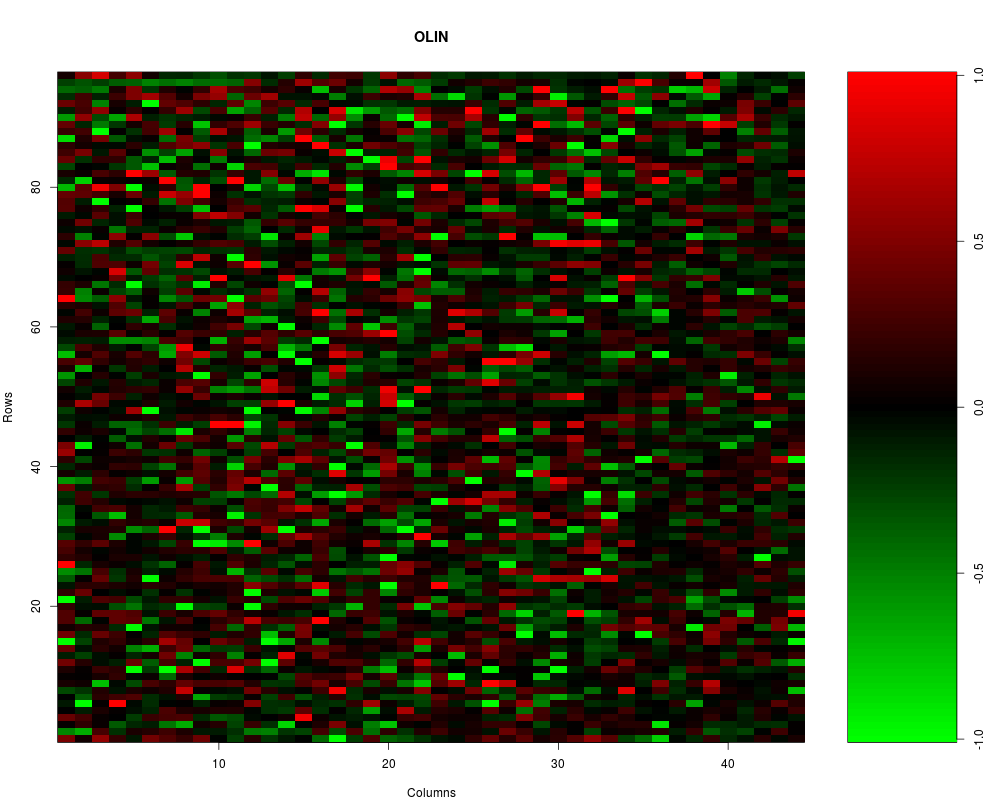
# CORRESPONDING MXY-PLOT
  mxy.plot(maM(norm.olin)[,1],Ngc=maNgc(norm.olin),Ngr=maNgr(norm.olin),
                Nsc=maNsc(norm.olin),Nsr=maNsr(norm.olin),main="OLIN")

# OPTIMISED SCALED LOCAL INTENSITY-DEPENDENT NORMALISATION
  norm.oslin <- olin(sw[,1],X=sw.xy$X[,1],Y=sw.xy$Y[,1],OSLIN=TRUE)
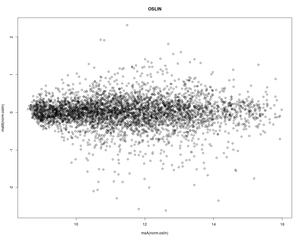
# MA-PLOT
  plot(maA(norm.oslin),maM(norm.oslin),main="OSLIN")
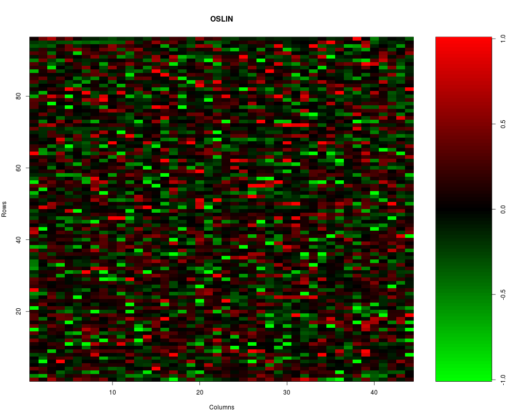
# MXY-PLOT
  mxy.plot(maM(norm.oslin)[,1],Ngc=maNgc(norm.oslin),Ngr=maNgr(norm.oslin),
                 Nsc=maNsc(norm.oslin),Nsr=maNsr(norm.oslin),main="OSLIN")

Results


R version 3.3.1 (2016-06-21) -- "Bug in Your Hair"
Copyright (C) 2016 The R Foundation for Statistical Computing
Platform: x86_64-pc-linux-gnu (64-bit)

R is free software and comes with ABSOLUTELY NO WARRANTY.
You are welcome to redistribute it under certain conditions.
Type 'license()' or 'licence()' for distribution details.

R is a collaborative project with many contributors.
Type 'contributors()' for more information and
'citation()' on how to cite R or R packages in publications.

Type 'demo()' for some demos, 'help()' for on-line help, or
'help.start()' for an HTML browser interface to help.
Type 'q()' to quit R.

> library(OLIN)
Loading required package: locfit
locfit 1.5-9.1 	 2013-03-22
Loading required package: marray
Loading required package: limma
> png(filename="/home/ddbj/snapshot/RGM3/R_BC/result/OLIN/olin.Rd_%03d_medium.png", width=480, height=480)
> ### Name: olin
> ### Title: Optimised local intensity-dependent normalisation of two-colour
> ###   microarrays
> ### Aliases: olin
> ### Keywords: utilities regression
> 
> ### ** Examples
> 
> 
> 
> # LOADING DATA
>   data(sw)
>   data(sw.xy)
> 
> # OPTIMISED LOCAL INTENSITY-DEPENDENT NORMALISATION OF FIRST ARRAY
>   norm.olin <- olin(sw[,1],X=sw.xy$X[,1],Y=sw.xy$Y[,1])
> 
> # MA-PLOT OF NORMALISATION RESULTS OF FIRST ARRAY
>   plot(maA(norm.olin),maM(norm.olin),main="OLIN")
>  
> # CORRESPONDING MXY-PLOT
>   mxy.plot(maM(norm.olin)[,1],Ngc=maNgc(norm.olin),Ngr=maNgr(norm.olin),
+                 Nsc=maNsc(norm.olin),Nsr=maNsr(norm.olin),main="OLIN")
> 
> # OPTIMISED SCALED LOCAL INTENSITY-DEPENDENT NORMALISATION
>   norm.oslin <- olin(sw[,1],X=sw.xy$X[,1],Y=sw.xy$Y[,1],OSLIN=TRUE)
> # MA-PLOT
>   plot(maA(norm.oslin),maM(norm.oslin),main="OSLIN")
> # MXY-PLOT
>   mxy.plot(maM(norm.oslin)[,1],Ngc=maNgc(norm.oslin),Ngr=maNgr(norm.oslin),
+                  Nsc=maNsc(norm.oslin),Nsr=maNsr(norm.oslin),main="OSLIN")
> 
> 
> 
> 
> 
> 
> dev.off()
null device 
          1 
>