Supported by Dr. Osamu Ogasawara and  . . |
|
Last data update: 2014.03.03 |
Functions for plotting matrices, or for splitting them and for maing suitable summariesDescription
Usage
  Mplot (M, ..., x = 1, select = NULL, which = select,
         subset = NULL, ask = NULL,
         legend = list(x = "center"), pos.legend = NULL,
         xyswap = FALSE, rev = "")

  Msummary (M, ...,
         select = NULL, which = select,
         subset = NULL)

  Mdescribe (M, ...,
         select = NULL, which = select,
         subset = NULL)

  Msplit (M, split = 1, subset = NULL)

  Mcommon (M, ..., verbose = FALSE)
Arguments
ValueFunction Function Function Function Author(s)Karline Soetaert <karline.soetaert@nioz.nl> Examples
# save plotting parameters
pm <- par("mfrow")
## =======================================================================
## Create three dummy matrices
## =======================================================================
M1 <- matrix(nrow = 10, ncol = 5, data = 1:50)
colnames(M1) <- LETTERS[1:5]
M2 <- M1[, c(1, 3, 4, 5, 2)]
M2[ ,-1] <- M2[,-1] /2
colnames(M2)[3] <- "CC" # Different name
M3 <- matrix(nrow = 5, ncol = 4, data = runif(20)*10)
M3[,1] <- sort(M3[,1])
colnames(M3) <- colnames(M1)[-3]
# show them
head(M1); head(M2); head(M3)
Msummary(M1)
Msummary(M1, M2, M3)
# plot all columns of M3 - will change mfrow
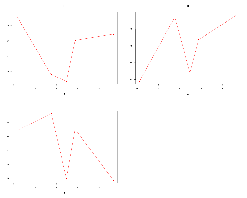
Mplot(M3, type = "b", pch = 18, col = "red")
# plot results of all three data sets
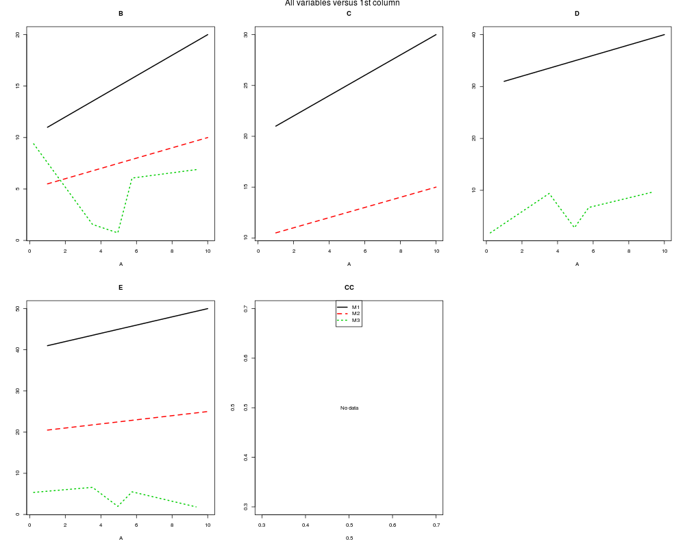
Mplot(M1, M2, M3, lwd = 2, mtext = "All variables versus 1st column",
legend = list(x = "top", legend = c("M1", "M2", "M3")))
## =======================================================================
## Plot a selection or only common elements
## =======================================================================
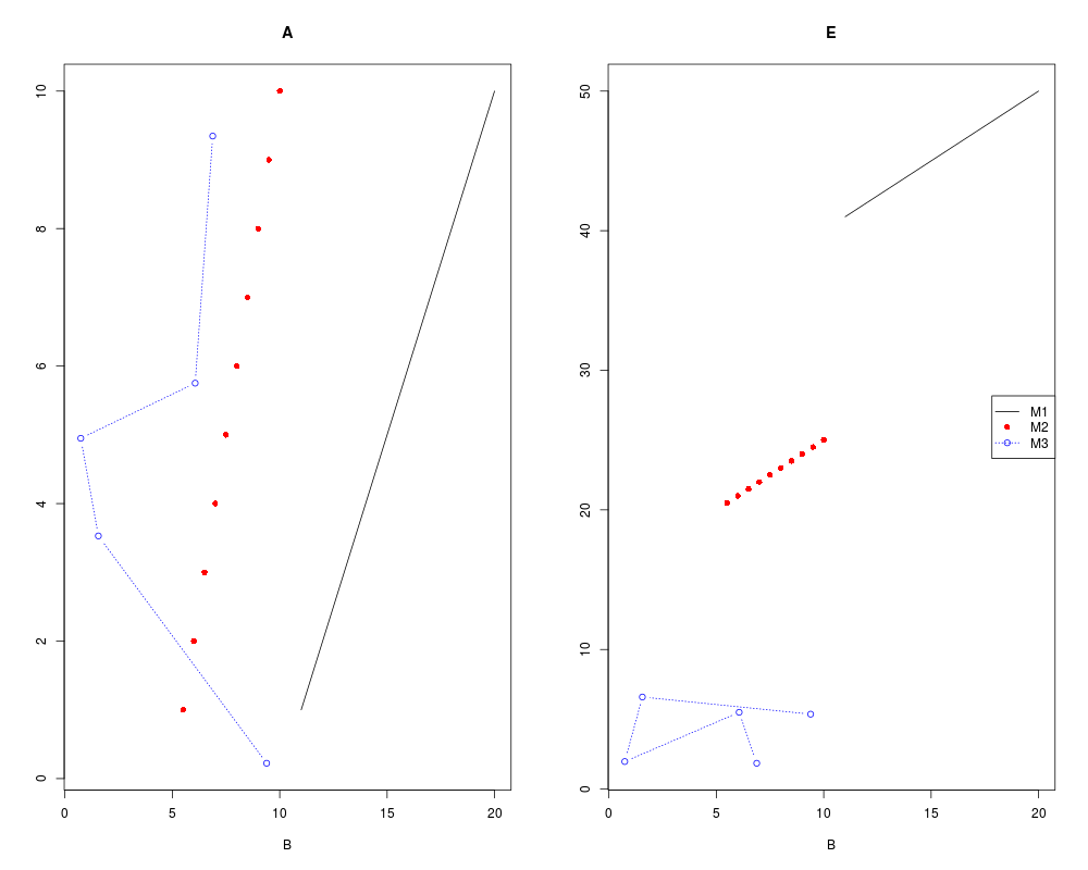
Mplot(M1, M2, M3, x = "B", select = c("A", "E"), pch = c(NA, 16, 1),
type = c("l", "p", "b"), col = c("black", "red", "blue"),
legend = list(x = "right", legend = c("M1", "M2", "M3")))
Mplot(Mcommon(M1, M2, M3), lwd = 2, mtext = "common variables",
legend = list(x = "top", legend = c("M1", "M2", "M3")))
Mdescribe(Mcommon(M1, M2, M3))
## =======================================================================
## The iris and Orange data set
## =======================================================================
# Split the matrix according to the species
Irislist <- Msplit(iris, split = "Species")
names(Irislist)
Mdescribe(Irislist, which = "Sepal.Length")
Mdescribe(iris, which = "Sepal.Length", subset = Species == "setosa")
# legend in a separate plot
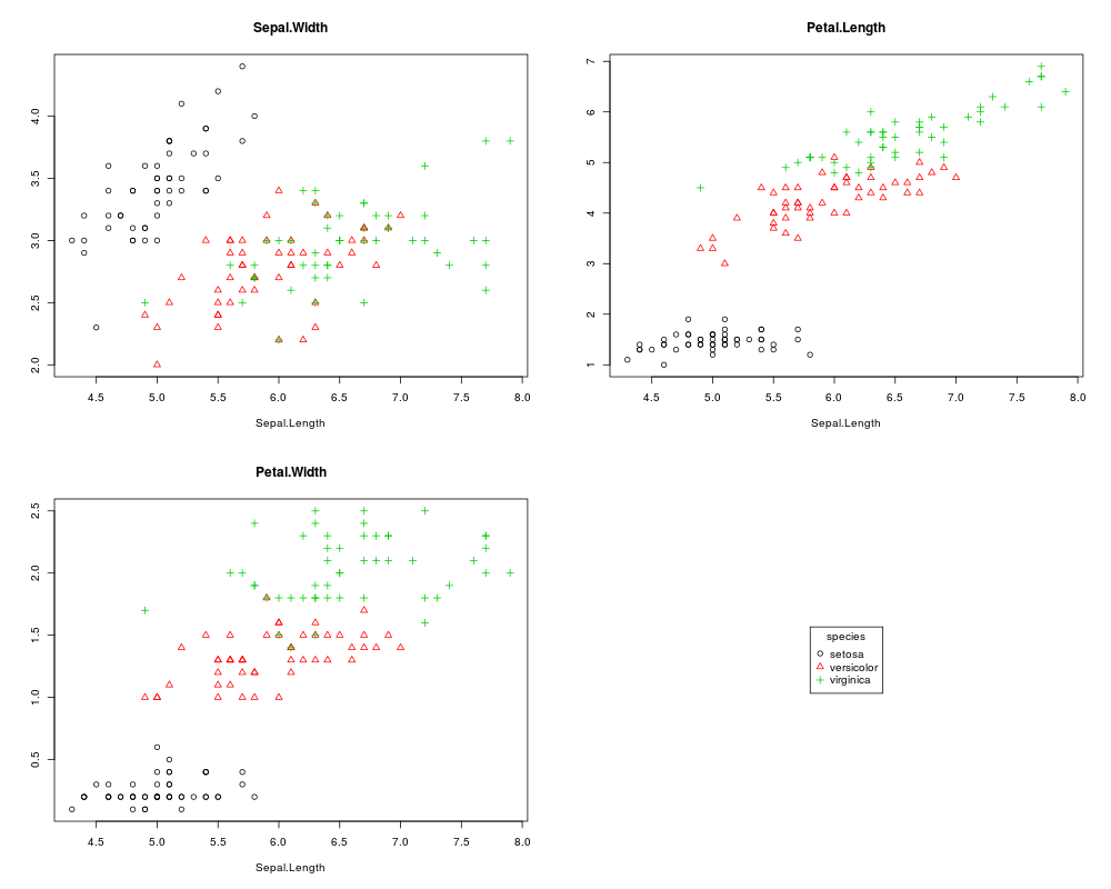
Mplot(Irislist, type = "p", pos.legend = 0,
legend = list(x = "center", title = "species"))
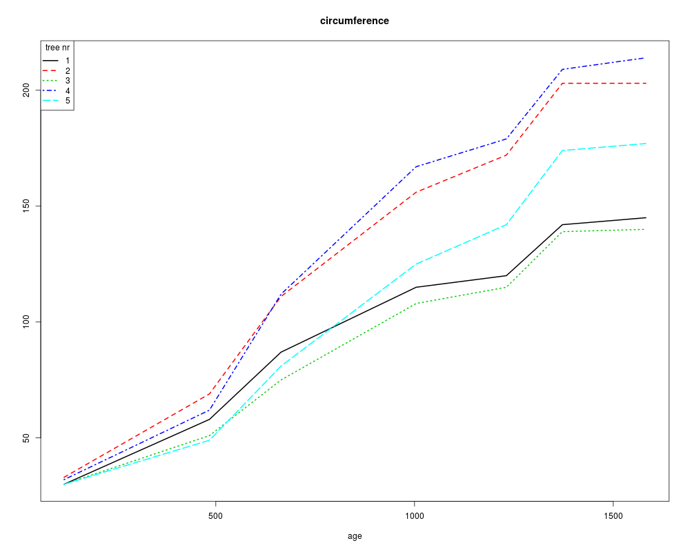
Mplot(Msplit(Orange,1), lwd = 2,
legend = list(x = "topleft", title = "tree nr"))
Msummary(Msplit(Orange,1))
# reset plotting parameters
par(mfrow = pm)
Results
R version 3.3.1 (2016-06-21) -- "Bug in Your Hair"
Copyright (C) 2016 The R Foundation for Statistical Computing
Platform: x86_64-pc-linux-gnu (64-bit)

R is free software and comes with ABSOLUTELY NO WARRANTY.
You are welcome to redistribute it under certain conditions.
Type 'license()' or 'licence()' for distribution details.

R is a collaborative project with many contributors.
Type 'contributors()' for more information and
'citation()' on how to cite R or R packages in publications.

Type 'demo()' for some demos, 'help()' for on-line help, or
'help.start()' for an HTML browser interface to help.
Type 'q()' to quit R.

> library(OceanView)
Loading required package: plot3D
Loading required package: plot3Drgl
Loading required package: rgl
> png(filename="/home/ddbj/snapshot/RGM3/R_CC/result/OceanView/Mplot.Rd_%03d_medium.png", width=480, height=480)
> ### Name: Matrix plotting
> ### Title: Functions for plotting matrices, or for splitting them and for
> ###   maing suitable summaries
> ### Aliases: Mplot Msplit Mcommon Msummary Mdescribe
> ### Keywords: hplot
>
> ### ** Examples
>
> # save plotting parameters
>  pm <- par("mfrow")
>
> ## =======================================================================
> ## Create three dummy matrices
> ## =======================================================================
>
>  M1 <- matrix(nrow = 10, ncol = 5, data = 1:50)
>  colnames(M1) <- LETTERS[1:5]
>
>  M2 <- M1[, c(1, 3, 4, 5, 2)]
>  M2[ ,-1] <- M2[,-1] /2
>  colnames(M2)[3] <- "CC"  # Different name
>
>  M3 <- matrix(nrow = 5, ncol = 4, data = runif(20)*10)
>  M3[,1] <- sort(M3[,1])
>  colnames(M3) <- colnames(M1)[-3]
>
> # show them
>  head(M1); head(M2); head(M3)
     A  B  C  D  E
[1,] 1 11 21 31 41
[2,] 2 12 22 32 42
[3,] 3 13 23 33 43
[4,] 4 14 24 34 44
[5,] 5 15 25 35 45
[6,] 6 16 26 36 46
     A    C   CC    E   B
[1,] 1 10.5 15.5 20.5 5.5
[2,] 2 11.0 16.0 21.0 6.0
[3,] 3 11.5 16.5 21.5 6.5
[4,] 4 12.0 17.0 22.0 7.0
[5,] 5 12.5 17.5 22.5 7.5
[6,] 6 13.0 18.0 23.0 8.0
             A        B        D        E
[1,] 0.8030771 6.810721 6.010145 5.379544
[2,] 1.8958684 2.319990 7.604166 0.783119
[3,] 2.7832681 5.937543 5.146703 8.699012
[4,] 2.8583299 9.111993 9.389603 8.761951
[5,] 4.5096555 7.796764 6.664586 8.254564
>  Msummary(M1)
  variable factor_or_char Min. X1st.Qu. Median Mean X3rd.Qu. Max.
1        A          FALSE    1     3.25    5.5  5.5     7.75   10
2        B          FALSE   11    13.25   15.5 15.5    17.75   20
3        C          FALSE   21    23.25   25.5 25.5    27.75   30
4        D          FALSE   31    33.25   35.5 35.5    37.75   40
5        E          FALSE   41    43.25   45.5 45.5    47.75   50
>  Msummary(M1, M2, M3)
   variable object factor_or_char       Min.  X1st.Qu.    Median      Mean
1         A     M1          FALSE  1.0000000  3.250000  5.500000  5.500000
2         A     M2          FALSE  1.0000000  3.250000  5.500000  5.500000
3         A     M3          FALSE  0.8030771  1.895868  2.783268  2.570040
4         B     M1          FALSE 11.0000000 13.250000 15.500000 15.500000
5         B     M2          FALSE  5.5000000  6.625000  7.750000  7.750000
6         B     M3          FALSE  2.3199897  5.937543  6.810721  6.395402
7         C     M1          FALSE 21.0000000 23.250000 25.500000 25.500000
8         C     M2          FALSE 10.5000000 11.625000 12.750000 12.750000
9         D     M1          FALSE 31.0000000 33.250000 35.500000 35.500000
10        D     M3          FALSE  5.1467028  6.010145  6.664586  6.963041
11        E     M1          FALSE 41.0000000 43.250000 45.500000 45.500000
12        E     M2          FALSE 20.5000000 21.625000 22.750000 22.750000
13        E     M3          FALSE  0.7831190  5.379544  8.254564  6.375638
14       CC     M2          FALSE 15.5000000 16.625000 17.750000 17.750000
    X3rd.Qu.      Max.
1   7.750000 10.000000
2   7.750000 10.000000
3   2.858330  4.509656
4  17.750000 20.000000
5   8.875000 10.000000
6   7.796764  9.111993
7  27.750000 30.000000
8  13.875000 15.000000
9  37.750000 40.000000
10  7.604166  9.389603
11 47.750000 50.000000
12 23.875000 25.000000
13  8.699012  8.761951
14 18.875000 20.000000
>
> # plot all columns of M3 -  will change mfrow
>  Mplot(M3, type = "b", pch = 18, col = "red")
>
> # plot results of all three data sets
>  Mplot(M1, M2, M3, lwd = 2, mtext = "All variables versus 1st column",
+        legend = list(x = "top", legend = c("M1", "M2", "M3")))
>
>
> ## =======================================================================
> ## Plot a selection or only common elements
> ## =======================================================================
>
>  Mplot(M1, M2, M3, x = "B", select = c("A", "E"), pch = c(NA, 16, 1),
+        type = c("l", "p", "b"), col = c("black", "red", "blue"),
+        legend = list(x = "right", legend = c("M1", "M2", "M3")))
>
>  Mplot(Mcommon(M1, M2, M3), lwd = 2, mtext = "common variables",
+        legend = list(x = "top", legend = c("M1", "M2", "M3")))
>
>  Mdescribe(Mcommon(M1, M2, M3))
  variable object factor_or_char  n missing unique      Mean       Sd
1        A     M1          FALSE 10       0     10  5.500000 3.027650
2        A     M2          FALSE 10       0     10  5.500000 3.027650
3        A     M3          FALSE  5       0      5  2.570040 1.366323
4        B     M1          FALSE 10       0     10 15.500000 3.027650
5        B     M2          FALSE 10       0     10  7.750000 1.513825
6        B     M3          FALSE  5       0      5  6.395402 2.565872
7        E     M1          FALSE 10       0     10 45.500000 3.027650
8        E     M2          FALSE 10       0     10 22.750000 1.513825
9        E     M3          FALSE  5       0      5  6.375638 3.423864
         Min     p0.05      p0.1      p0.5      p0.9     p0.95       Max
1  1.0000000  1.450000  1.900000  5.500000  9.100000  9.550000 10.000000
2  1.0000000  1.450000  1.900000  5.500000  9.100000  9.550000 10.000000
3  0.8030771  1.021635  1.240194  2.783268  3.849125  4.179390  4.509656
4 11.0000000 11.450000 11.900000 15.500000 19.100000 19.550000 20.000000
5  5.5000000  5.725000  5.950000  7.750000  9.550000  9.775000 10.000000
6  2.3199897  3.043500  3.767011  6.810721  8.585902  8.848948  9.111993
7 41.0000000 41.450000 41.900000 45.500000 49.100000 49.550000 50.000000
8 20.5000000 20.725000 20.950000 22.750000 24.550000 24.775000 25.000000
9  0.7831190  1.702404  2.621689  8.254564  8.736775  8.749363  8.761951
>
> ## =======================================================================
> ## The iris and Orange data set
> ## =======================================================================
>
> # Split the matrix according to the species
>  Irislist <- Msplit(iris, split = "Species")
>  names(Irislist)
[1] "setosa"     "versicolor" "virginica"
>
>  Mdescribe(Irislist, which = "Sepal.Length")
      variable     object factor_or_char  n missing unique  Mean        Sd Min
1 Sepal.Length     setosa          FALSE 50       0     15 5.006 0.3524897 4.3
2 Sepal.Length versicolor          FALSE 50       0     21 5.936 0.5161711 4.9
3 Sepal.Length  virginica          FALSE 50       0     21 6.588 0.6358796 4.9
  p0.05 p0.1 p0.5 p0.9 p0.95 Max
1 4.400 4.59  5.0 5.41 5.610 5.8
2 5.045 5.38  5.9 6.70 6.755 7.0
3 5.745 5.80  6.5 7.61 7.700 7.9
>  Mdescribe(iris, which = "Sepal.Length", subset = Species == "setosa")
      variable factor_or_char  n missing unique  Mean        Sd Min p0.05 p0.1
1 Sepal.Length          FALSE 50       0     15 5.006 0.3524897 4.3   4.4 4.59
  p0.5 p0.9 p0.95 Max
1    5 5.41  5.61 5.8
>
> # legend in a separate plot
>  Mplot(Irislist, type = "p", pos.legend = 0,
+        legend = list(x = "center", title = "species"))
>
>  Mplot(Msplit(Orange,1), lwd = 2,
+        legend = list(x = "topleft", title = "tree nr"))
>  Msummary(Msplit(Orange,1))
        variable object factor_or_char Min. X1st.Qu. Median      Mean X3rd.Qu.
1            age      1          FALSE  118    574.0   1004 922.14286   1301.5
2            age      2          FALSE  118    574.0   1004 922.14286   1301.5
3            age      3          FALSE  118    574.0   1004 922.14286   1301.5
4            age      4          FALSE  118    574.0   1004 922.14286   1301.5
5            age      5          FALSE  118    574.0   1004 922.14286   1301.5
6  circumference      1          FALSE   30     72.5    115  99.57143    131.0
7  circumference      2          FALSE   33     90.0    156 135.28571    187.5
8  circumference      3          FALSE   30     63.0    108  94.00000    127.0
9  circumference      4          FALSE   32     87.0    167 139.28571    194.0
10 circumference      5          FALSE   30     65.0    125 111.14286    158.0
   Max.
1  1582
2  1582
3  1582
4  1582
5  1582
6   145
7   203
8   140
9   214
10  177
>
> # reset plotting parameters
>  par(mfrow = pm)
>
>
>
>
>
> dev.off()
null device
          1
>
|