Supported by Dr. Osamu Ogasawara and  . . |
|
Last data update: 2014.03.03 |
Plotting tracer distributions in 3DDescription
It is based on the Usage
  tracers3D (x, y, z, colvar = NULL, ...,
      col = NULL, NAcol = "white", breaks = NULL,
      colkey = FALSE, clim = NULL, clab = NULL, surf = NULL)

  tracers3Drgl (x, y, z, colvar = NULL, ...,
      col = NULL, NAcol = "white", breaks = NULL,
      colkey = FALSE, clim = NULL, clab = NULL)

  moviepoints3D (x, y, z, colvar, t, by = 1,
    col = jet.col(100), NAcol = "white", breaks = NULL,
    clim = NULL, wait  = NULL, ask = FALSE, add = FALSE,
    basename = NULL, ...)
Arguments
Valuereturns nothing Author(s)Karline Soetaert <karline.soetaert@nioz.nl> See Alsotracers2D for plotting time series of tracer distributions in 2D movieslice3D for plotting slices in 3D Ltrans for 3-D output of a particle tracking model Examples
# save plotting parameters
pm <- par("mfrow")
## =======================================================================
## Create topography, data
## =======================================================================
# The topographic surface
x <- seq(-pi, pi, by = 0.2)
y <- seq(0, pi, by = 0.1)
M <- mesh(x, y)
z <- with(M, sin(x)*sin(y))
# Initial condition
xi <- c(0.25 * rnorm(100) - pi/2, 0.25 * rnorm(100) - pi/4)
yi <- 0.25 * rnorm(200) + pi/2
zi <- 0.005*rnorm(200) + 0.5
# the species
species <- c(rep(1, 100), rep(2, 100))
# set initial conditions
xp <- xi; yp <- yi; zp <- zi
## =======================================================================
## Traditional graphics
## =======================================================================
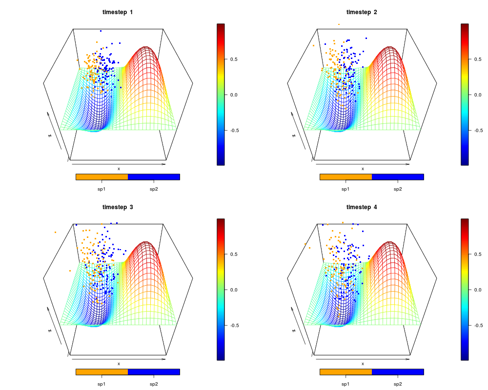
par(mfrow = c(2, 2))
# Topography is defined by argument surf
for (i in 1:4) {
# update tracer distribution
xp <- xp + 0.25 * rnorm(200)
yp <- yp + 0.025 * rnorm(200)
zp <- zp + 0.25 *rnorm(200)
# plot new tracer distribution
tracers3D(xp, yp, zp, colvar = species, pch = ".", cex = 5,
main = paste("timestep ", i), col = c("orange", "blue"),
surf = list(x, y, z = z, theta = 0, facets = FALSE),
colkey = list(side = 1, length = 0.5, labels = c("sp1","sp2"),
at = c(1.25, 1.75), dist = 0.075))
}
# same, but creating topography first
## Not run:
# create the topography on which to add points
persp3D(x, y, z = z, theta = 0, facets = FALSE, plot = FALSE)
for (i in 1:4) {
# update tracer distribution
xp <- xp + 0.25 * rnorm(200)
yp <- yp + 0.025 * rnorm(200)
zp <- zp + 0.25 *rnorm(200)
# plot new tracer distribution
tracers3D(xp, yp, zp, colvar = species, pch = ".", cex = 5,
main = paste("timestep ", i), col = c("orange", "blue"),
colkey = list(side = 1, length = 0.5, labels = c("sp1","sp2"),
at = c(1.25, 1.75), dist = 0.075))
}
## End(Not run)
## =======================================================================
## rgl graphics
## =======================================================================
# pause <- 0.05
# create a suitable topography
persp3D(x, y, z = z, theta = 0, facets = NA, plot = FALSE)
plotrgl( )
xp <- xi; yp <- yi; zp <- zi
nstep <- 10
for (i in 1:nstep) {
xp <- xp + 0.05 * rnorm(200) + 0.05
yp <- yp + 0.0025 * (rnorm(200) + 0.0025)
zp <- zp + 0.05 *rnorm(200)
# tracers3Drgl(xp, yp, zp, col = c(rep("orange", 100), rep("blue", 100)),
# main = paste("timestep ", i))
# or:
tracers3Drgl(xp, yp, zp, colvar = species, col = c("orange", "blue"),
main = paste("timestep ", i))
# Sys.sleep(pause)
# or: readline("hit enter for next")
}
# using function moviepoints3D
## Not run:
# first create the data in matrices
xp <- matrix(nrow = 200, ncol = nstep, data = xi)
yp <- matrix(nrow = 200, ncol = nstep, data = yi)
zp <- matrix(nrow = 200, ncol = nstep, data = zi)
tp <- matrix(nrow = 200, ncol = nstep, data = 0)
cv <- matrix(nrow = 200, ncol = nstep, data = species)
nstep <- 10
for (i in 2:nstep) {
xp[,i] <- xp[,i-1] + 0.05 * rnorm(200) + 0.05
yp[,i] <- yp[,i-1] + 0.0025 * (rnorm(200) + 0.0025)
zp[,i] <- zp[,i-1] + 0.05 *rnorm(200)
tp[,i] <- i
}
# create the topography
persp3Drgl(x, y, z = z, theta = 0, lighting = TRUE, smooth = TRUE)
# add moviepoints:
moviepoints3D (xp, yp, zp, colvar = cv, t = tp,
wait = 0.05, cex = 10, col = c("red", "orange"))
## End(Not run)
# reset plotting parameters
par(mfrow = pm)
Results
R version 3.3.1 (2016-06-21) -- "Bug in Your Hair"
Copyright (C) 2016 The R Foundation for Statistical Computing
Platform: x86_64-pc-linux-gnu (64-bit)

R is free software and comes with ABSOLUTELY NO WARRANTY.
You are welcome to redistribute it under certain conditions.
Type 'license()' or 'licence()' for distribution details.

R is a collaborative project with many contributors.
Type 'contributors()' for more information and
'citation()' on how to cite R or R packages in publications.

Type 'demo()' for some demos, 'help()' for on-line help, or
'help.start()' for an HTML browser interface to help.
Type 'q()' to quit R.

> library(OceanView)
Loading required package: plot3D
Loading required package: plot3Drgl
Loading required package: rgl
> png(filename="/home/ddbj/snapshot/RGM3/R_CC/result/OceanView/tracers3D.Rd_%03d_medium.png", width=480, height=480)
> ### Name: Tracers in 3D
> ### Title: Plotting tracer distributions in 3D
> ### Aliases: tracers3D tracers3Drgl moviepoints3D
> ### Keywords: hplot
>
> ### ** Examples
>
> # save plotting parameters
>  pm <- par("mfrow")
>
> ## =======================================================================
> ## Create topography, data
> ## =======================================================================
>
> # The topographic surface
>  x <-  seq(-pi, pi, by = 0.2)
>  y <-  seq(0, pi, by = 0.1)
>  M <- mesh(x, y)
>  z <- with(M, sin(x)*sin(y))
>
> # Initial condition
>  xi <- c(0.25 * rnorm(100) - pi/2, 0.25 * rnorm(100) - pi/4)
>  yi <- 0.25 * rnorm(200) + pi/2
>  zi <- 0.005*rnorm(200) + 0.5
>
> # the species
>  species <- c(rep(1, 100), rep(2, 100))
>
> # set initial conditions
>  xp <- xi; yp <- yi; zp <- zi
>
> ## =======================================================================
> ## Traditional graphics
> ## =======================================================================
>
>  par(mfrow = c(2, 2))
>
> # Topography is defined by argument surf
>  for (i in 1:4) {
+   # update tracer distribution
+    xp <- xp + 0.25 * rnorm(200)
+    yp <- yp + 0.025 * rnorm(200)
+    zp <- zp + 0.25 *rnorm(200)
+
+   # plot new tracer distribution
+    tracers3D(xp, yp, zp, colvar = species, pch = ".", cex = 5,
+      main = paste("timestep ", i), col = c("orange", "blue"),
+      surf = list(x, y, z = z, theta = 0, facets = FALSE),
+      colkey = list(side = 1, length = 0.5, labels = c("sp1","sp2"),
+                    at = c(1.25, 1.75), dist = 0.075))
+  }
>
> # same, but creating topography first
> ## Not run:
> ##D # create the topography on which to add points
> ##D  persp3D(x, y, z = z, theta = 0, facets = FALSE, plot = FALSE)
> ##D
> ##D  for (i in 1:4) {
> ##D   # update tracer distribution
> ##D    xp <- xp + 0.25 * rnorm(200)
> ##D    yp <- yp + 0.025 * rnorm(200)
> ##D    zp <- zp + 0.25 *rnorm(200)
> ##D
> ##D   # plot new tracer distribution
> ##D    tracers3D(xp, yp, zp, colvar = species, pch = ".", cex = 5,
> ##D      main = paste("timestep ", i), col = c("orange", "blue"),
> ##D      colkey = list(side = 1, length = 0.5, labels = c("sp1","sp2"),
> ##D                     at = c(1.25, 1.75), dist = 0.075))
> ##D  }
> ## End(Not run)
>
> ## =======================================================================
> ## rgl graphics
> ## =======================================================================
>
> # pause <- 0.05
> # create a suitable topography
>  persp3D(x, y, z = z, theta = 0, facets = NA, plot = FALSE)
>
>  plotrgl( )
>  xp <- xi; yp <- yi; zp <- zi
>
>  nstep <- 10
>  for (i in 1:nstep) {
+    xp <- xp + 0.05 * rnorm(200) + 0.05
+    yp <- yp + 0.0025 * (rnorm(200) + 0.0025)
+    zp <- zp + 0.05 *rnorm(200)
+
+ #   tracers3Drgl(xp, yp, zp, col = c(rep("orange", 100), rep("blue", 100)),
+ #     main = paste("timestep ", i))
+ # or:
+    tracers3Drgl(xp, yp, zp, colvar = species, col = c("orange", "blue"),
+      main = paste("timestep ", i))
+ #   Sys.sleep(pause)
+ # or:  readline("hit enter for next")
+  }
>
> # using function moviepoints3D
>
> ## Not run:
> ##D # first create the data in matrices
> ##D  xp <- matrix(nrow = 200, ncol = nstep, data = xi)
> ##D  yp <- matrix(nrow = 200, ncol = nstep,  data = yi)
> ##D  zp <- matrix(nrow = 200, ncol = nstep, data = zi)
> ##D  tp <- matrix(nrow = 200, ncol = nstep, data = 0)
> ##D  cv <- matrix(nrow = 200, ncol = nstep, data = species)
> ##D  nstep <- 10
> ##D  for (i in 2:nstep) {
> ##D    xp[,i] <- xp[,i-1] + 0.05 * rnorm(200) + 0.05
> ##D    yp[,i] <- yp[,i-1] + 0.0025 * (rnorm(200) + 0.0025)
> ##D    zp[,i] <- zp[,i-1] + 0.05 *rnorm(200)
> ##D    tp[,i] <- i
> ##D  }
> ##D # create the topography
> ##D  persp3Drgl(x, y, z = z, theta = 0, lighting = TRUE, smooth = TRUE)
> ##D
> ##D # add moviepoints:
> ##D   moviepoints3D (xp, yp, zp, colvar = cv, t = tp,
> ##D     wait = 0.05, cex = 10, col = c("red", "orange"))
> ##D
> ## End(Not run)
>
> # reset plotting parameters
>  par(mfrow = pm)
>
>
>
>
>
> dev.off()
null device
          1
>
|