R Graphical Manual

Browse All

Last data update: 2014.03.03

R: Compare balance graphically of a continuous covariate as part...

box.psa

R Documentation

Compare balance graphically of a continuous covariate as part of a PSA

Description

Given predefined strata and two level treatment for a continuous covariate from a propensity score analysis, box.psa draws pairs of side by side boxplots corresponding to control and treatment for each stratum.

Usage

box.psa(continuous, treatment = NULL, strata = NULL, boxwex = 0.17, 
offset = 0.17, 
col = c("yellow", "orange", "black", "red", "darkorange3"),
xlab = "Stratum", legend.xy = NULL, 
legend.labels = NULL, pts = TRUE, 
balance = FALSE, trim = 0, B = 1000, ...)

Arguments

`continuous`	Vector or N X 3 dataframe or matrix. If a vector, then represents the quantitative covariate that is being balanced within strata in a PSA. If `continuous` has three columns, then the second and third are assumed to be the `treatment` and `strata` respectively. Missing values are not allowed.
`treatment`	Binary vector of same length as `continuous` representing the two treatments; can be a character vector or factor.
`strata`	A vector or factor of same length as `continuous` indicating the derived strata from estimated propensity scores. May be numeric or character vector, or factor. Strata are ordered lexicographically in plot.
`boxwex`	Numeric; controls width of boxes. Default = 0.17
`offset`	Numeric; controls distance between the two boxes in each stratum. Default = 0.17
`col`	Default = `c("yellow", "orange", "black", "red", "darkorange3")`. Color vector for the control boxes, treatment boxes, and line connecting their means.
`xlab`	Label for the x-axis; default = `"Stratum"`. Other standard labels may be used as well.
`legend.xy`	Binary vector giving coordinates of the legend. By default the legend is placed to the top left.
`legend.labels`	Vector of labels for the legend; default is essentially `c("Treatment (first)", "Treatment (second)", "Treatment Means Compared", "KS p-values", "Strata-Treatment Size")` where treatment names are taken from `treatment`. Vector has four elements if `balance = FALSE`, ommitting "KS p-values".
`pts`	Logical; if `TRUE` then (jittered) points are added on top of the boxplots.
`balance`	Logical; if `TRUE` then `bal.ms.psa` provides a histogram of a permutation distribution and reference statstic to assess balance across strata; `bal.ks.psa` adds p-values to the graph derived from 2-sample Kologmorov-Smirnov tests of equivalence of control/treatment distributions within each stratum.
`trim`	If `balance=TRUE`, defines fraction (0 to 0.5) of observations to be trimmed from each end of stratum-treatment level before the mean is computed. See `mean`, `bal.ms.psa`.
`B`	Passed to `bal.ms.psa` if necessary, determines number of randomly generated comparison statistics. Default =1000.
`...`	Other graphical parameters passed to `boxplot`.

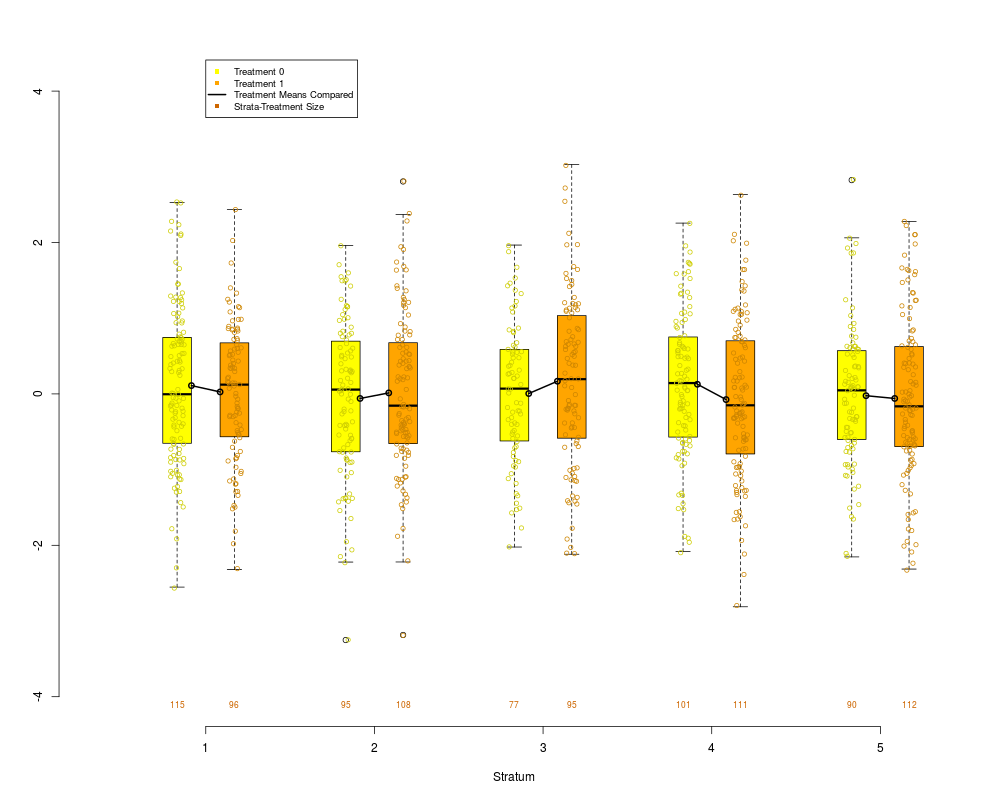
Details

Draws a pair of side by side boxplots for each stratum of a propensity score analysis. This allows visual comparisons within strata of the distribution of the given continuous covariate, and comparisons between strata as well. The number of observations in each boxplot are given below each box, and the means of paired treatment and control groups are connected.

Author(s)

James E. Helmreich James.Helmreich@Marist.edu

Robert M. Pruzek RMPruzek@yahoo.com

Examples

 
continuous<-rnorm(1000)
treatment<-sample(c(0,1),1000,replace=TRUE)
strata<-sample(5,1000,replace=TRUE)
box.psa(continuous, treatment, strata)

data(lindner)
attach(lindner)
lindner.ps <- glm(abcix ~ stent + height + female + 
      diabetic + acutemi + ejecfrac + ves1proc, 
      data = lindner, family = binomial)
ps<-lindner.ps$fitted
lindner.s5 <- as.numeric(cut(ps, quantile(ps, seq(0, 1, 1/5)),
      include.lowest = TRUE, labels = FALSE))
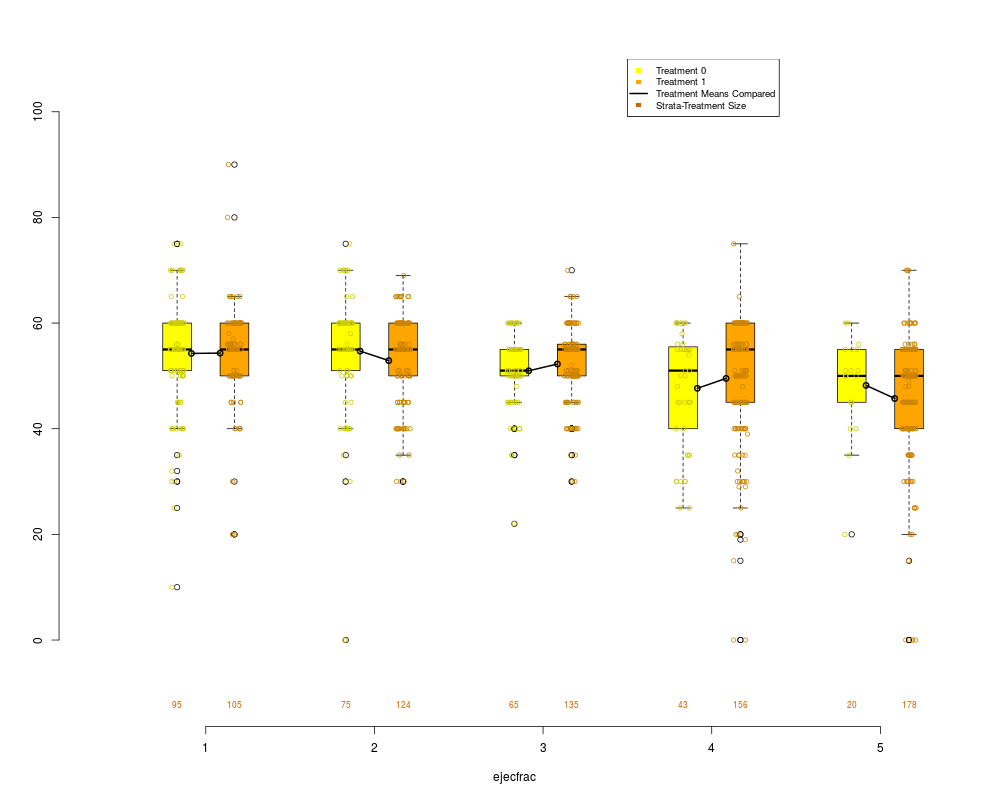
box.psa(ejecfrac, abcix, lindner.s5, xlab = "ejecfrac", 
      legend.xy = c(3.5,110))

lindner.s10 <- as.numeric(cut(ps, quantile(ps, seq(0, 1, 1/5)),
      include.lowest = TRUE, labels = FALSE))
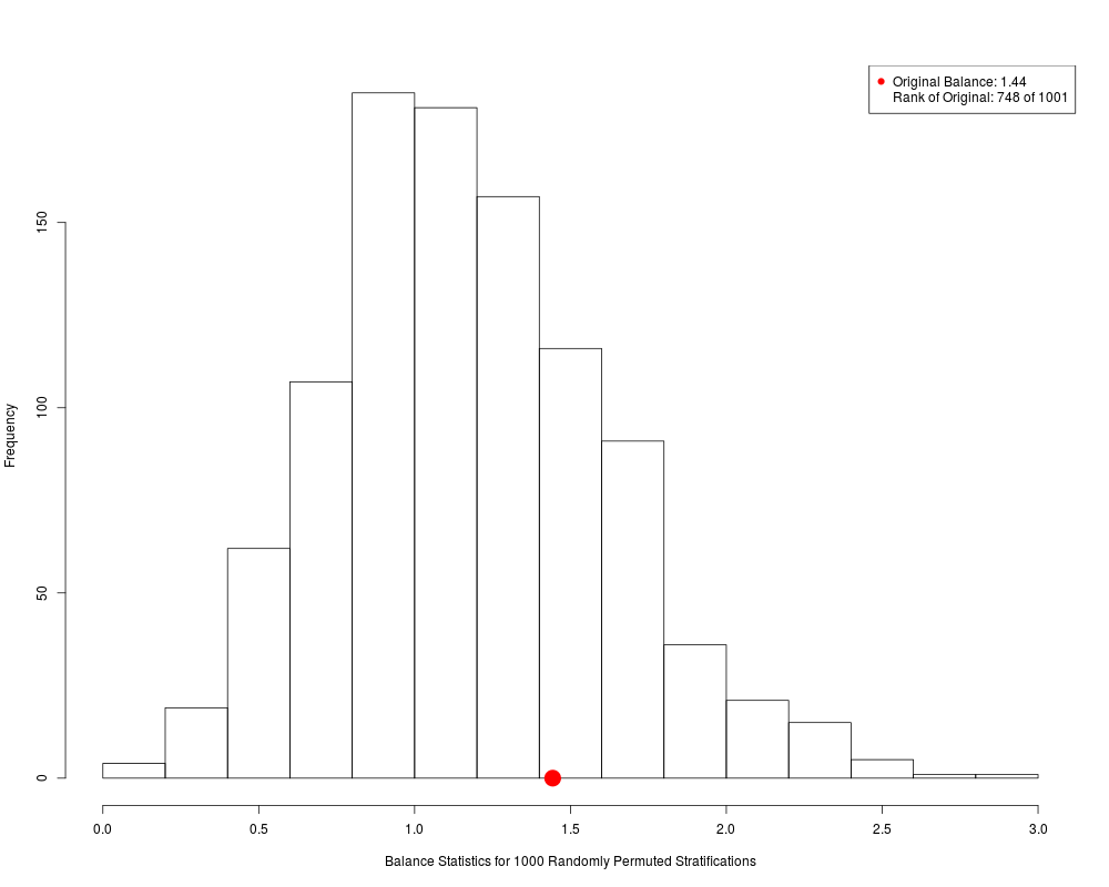
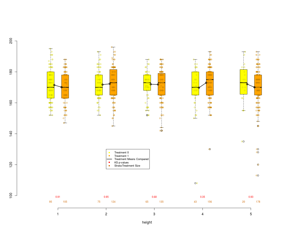
box.psa(height, abcix, lindner.s10, xlab="height", 
      boxwex = .15, offset = .15, legend.xy = c(2,130), balance = TRUE)

Results


R version 3.3.1 (2016-06-21) -- "Bug in Your Hair"
Copyright (C) 2016 The R Foundation for Statistical Computing
Platform: x86_64-pc-linux-gnu (64-bit)

R is free software and comes with ABSOLUTELY NO WARRANTY.
You are welcome to redistribute it under certain conditions.
Type 'license()' or 'licence()' for distribution details.

R is a collaborative project with many contributors.
Type 'contributors()' for more information and
'citation()' on how to cite R or R packages in publications.

Type 'demo()' for some demos, 'help()' for on-line help, or
'help.start()' for an HTML browser interface to help.
Type 'q()' to quit R.

> library(PSAgraphics)
Loading required package: rpart
> png(filename="/home/ddbj/snapshot/RGM3/R_CC/result/PSAgraphics/box.psa.Rd_%03d_medium.png", width=480, height=480)
> ### Name: box.psa
> ### Title: Compare balance graphically of a continuous covariate as part of
> ###   a PSA
> ### Aliases: box.psa
> ### Keywords: hplot htest
> 
> ### ** Examples
>  
> continuous<-rnorm(1000)
> treatment<-sample(c(0,1),1000,replace=TRUE)
> strata<-sample(5,1000,replace=TRUE)
> box.psa(continuous, treatment, strata)
Warning messages:
1: In xy.coords(x, y) : NAs introduced by coercion
2: In xy.coords(x, y) : NAs introduced by coercion
> 
> data(lindner)
> attach(lindner)
> lindner.ps <- glm(abcix ~ stent + height + female + 
+       diabetic + acutemi + ejecfrac + ves1proc, 
+       data = lindner, family = binomial)
> ps<-lindner.ps$fitted
> lindner.s5 <- as.numeric(cut(ps, quantile(ps, seq(0, 1, 1/5)),
+       include.lowest = TRUE, labels = FALSE))
> box.psa(ejecfrac, abcix, lindner.s5, xlab = "ejecfrac", 
+       legend.xy = c(3.5,110))
Warning messages:
1: In xy.coords(x, y) : NAs introduced by coercion
2: In xy.coords(x, y) : NAs introduced by coercion
> 
> lindner.s10 <- as.numeric(cut(ps, quantile(ps, seq(0, 1, 1/5)),
+       include.lowest = TRUE, labels = FALSE))
> box.psa(height, abcix, lindner.s10, xlab="height", 
+       boxwex = .15, offset = .15, legend.xy = c(2,130), balance = TRUE)
Press <enter> for bar chart...
Warning messages:
1: In ks.test(continuous[treatment == unique(treatment)[1] & strat.f ==  :
  cannot compute exact p-value with ties
2: In ks.test(continuous[treatment == unique(treatment)[1] & strat.f ==  :
  cannot compute exact p-value with ties
3: In ks.test(continuous[treatment == unique(treatment)[1] & strat.f ==  :
  cannot compute exact p-value with ties
4: In ks.test(continuous[treatment == unique(treatment)[1] & strat.f ==  :
  cannot compute exact p-value with ties
5: In ks.test(continuous[treatment == unique(treatment)[1] & strat.f ==  :
  cannot compute exact p-value with ties
6: In xy.coords(x, y) : NAs introduced by coercion
7: In xy.coords(x, y) : NAs introduced by coercion
> 
> 
> 
> 
> 
> dev.off()
null device 
          1 
>