Supported by Dr. Osamu Ogasawara and  . . |
|
Last data update: 2014.03.03 |
Multiple Covariate Balance Assessment PlotDescriptionProvides a graphic that depicts covarite effect size differences between treatment groups both before and after stratification. Function will create stata internally if desired, and returns numerical output used to create graphic. Usagecv.bal.psa(covariates, treatment, propensity, strata = NULL, int = NULL, tree = FALSE, minsize = 2, universal.psd = TRUE, trM = 0, absolute.es = TRUE, trt.value = NULL, use.trt.var = FALSE, verbose = FALSE, xlim = NULL, plot.strata = TRUE, ...) Arguments
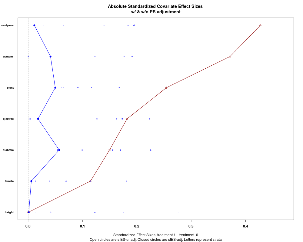
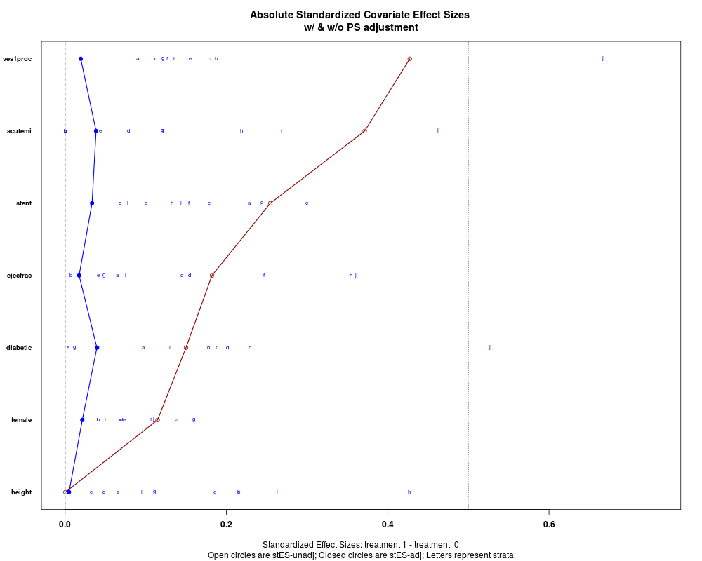
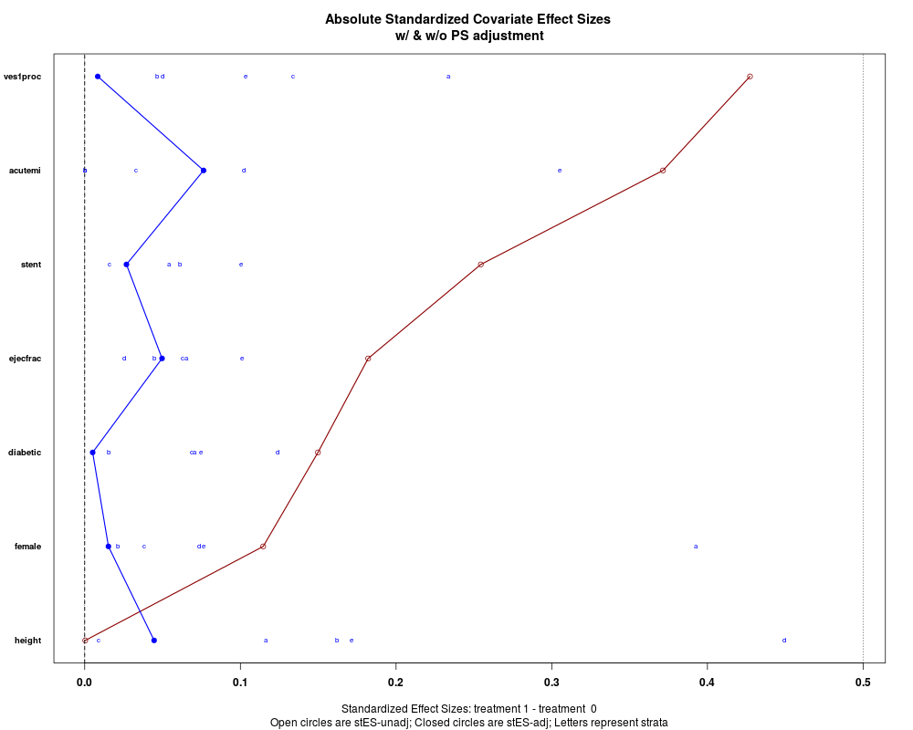
DetailsEffect sizes between treatments for each covariate are presented in one graphic, both before and after stratification. ValueGraphic plots covariate balance before and after stratication on propensity scores.
The default version (absolute.es = TRUE) plots the absolute values of effect sizes for each stratum, though the
overall estimate is the weighted mean before taking the absolute values.
Numerical output consists of seven addressable objects. If
Author(s)Robert M. Pruzek RMPruzek@yahoo.com James E. Helmreich James.Helmreich@Marist.edu KuangNan Xiong harryxkn@yahoo.com References“Matching Methods for Causal Inference: A review and a look forward." Forthcoming in Statistical Science. See Also
Examples
data(lindner)
attach(lindner)
lindner.ps <- glm(abcix ~ stent + height + female +
      diabetic + acutemi + ejecfrac + ves1proc,
      data = lindner, family = binomial)
ps<-lindner.ps$fitted
lindner.cv <- lindner[,4:10]
cv.bal.psa(lindner.cv, abcix, ps, strata = 5)
cv.bal.psa(lindner.cv, abcix, ps, strata = 10)
cv.bal.psa(lindner.cv, abcix, ps, int = c(.2, .5, .6, .75, .8))
Results
R version 3.3.1 (2016-06-21) -- "Bug in Your Hair"
Copyright (C) 2016 The R Foundation for Statistical Computing
Platform: x86_64-pc-linux-gnu (64-bit)

R is free software and comes with ABSOLUTELY NO WARRANTY.
You are welcome to redistribute it under certain conditions.
Type 'license()' or 'licence()' for distribution details.

R is a collaborative project with many contributors.
Type 'contributors()' for more information and
'citation()' on how to cite R or R packages in publications.

Type 'demo()' for some demos, 'help()' for on-line help, or
'help.start()' for an HTML browser interface to help.
Type 'q()' to quit R.

> library(PSAgraphics)
Loading required package: rpart
> png(filename="/home/ddbj/snapshot/RGM3/R_CC/result/PSAgraphics/cv.bal.psa.Rd_%03d_medium.png", width=480, height=480)
> ### Name: cv.bal.psa
> ### Title: Multiple Covariate Balance Assessment Plot
> ### Aliases: cv.bal.psa
> ### Keywords: hplot
>
> ### ** Examples
>
> data(lindner)
> attach(lindner)
> lindner.ps <- glm(abcix ~ stent + height + female +
+       diabetic + acutemi + ejecfrac + ves1proc,
+       data = lindner, family = binomial)
> ps<-lindner.ps$fitted
> lindner.cv <- lindner[,4:10]
> cv.bal.psa(lindner.cv, abcix, ps, strata = 5)
> cv.bal.psa(lindner.cv, abcix, ps, strata = 10)
> cv.bal.psa(lindner.cv, abcix, ps, int = c(.2, .5, .6, .75, .8))
>
>
>
>
>
> dev.off()
null device
          1
>
|