Makes formatted plots from the clustering result returned
from ClusProc.
Usage
  ## S3 method for class 'clust'
 plot(x,
    type = c("histo", "scat", "sil"), adjust = TRUE, ...)
Arguments
x
The clustering results obtained from
ClusProc.
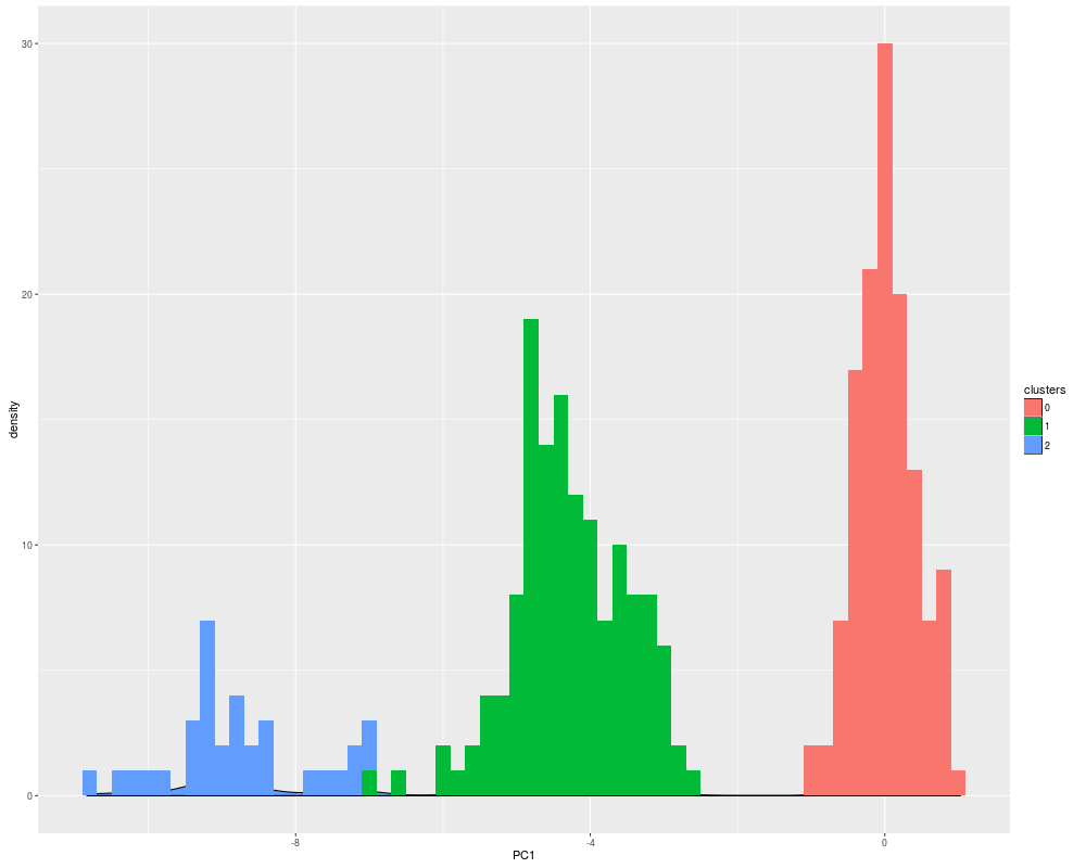
type
Factor. For specifying the plot type. It must
be one of 'histo', 'scat' and 'sil'. If it is 'histo',
the histogram is obtained with the first PC score of the
intensity measurement. For 'scat', the first PC score of
the intensity measurement is plotted against the mean of
the intensity measurement. For 'sil', the silhouette
score is plotted. See details.
adjust
Logicals. If TRUE (default), the
silhouette-adjusted clustering result will be used. If
FALSE, the initial clustering result will be used. See
details in ClusProc.
...
Usual arguments passed to the qplot function.
Details
typeWe provide three types of plots:
'hist', 'scat' and 'sil'. The first two plots are used to
visually check the performance of clustering. Different
clusters are represented by using different colors. The
'sil' plot is the the overview of the silhouette value
for all the individuals, the silhouettes of the different
clusters are printed below each other. The higher
silhouettes value means the better performance.
Author(s)
Meiling Liu
Examples
# Fit the data under the given clustering numbers
clus.fit <- ClusProc(signal=signal,N=2:6,varSelection='PC.9')
plot(clus.fit,type='histo')
Results
R version 3.3.1 (2016-06-21) -- "Bug in Your Hair"
Copyright (C) 2016 The R Foundation for Statistical Computing
Platform: x86_64-pc-linux-gnu (64-bit)

R is free software and comes with ABSOLUTELY NO WARRANTY.
You are welcome to redistribute it under certain conditions.
Type 'license()' or 'licence()' for distribution details.

R is a collaborative project with many contributors.
Type 'contributors()' for more information and
'citation()' on how to cite R or R packages in publications.

Type 'demo()' for some demos, 'help()' for on-line help, or
'help.start()' for an HTML browser interface to help.
Type 'q()' to quit R.

> library(PedCNV)
Loading required package: Rcpp
Loading required package: RcppArmadillo
Loading required package: ggplot2
> png(filename="/home/ddbj/snapshot/RGM3/R_CC/result/PedCNV/plot.clust.Rd_%03d_medium.png", width=480, height=480)
> ### Name: plot.clust
> ### Title: Plots clustering result
> ### Aliases: plot.clust
>
> ### ** Examples
>
> # Fit the data under the given clustering numbers
> clus.fit <- ClusProc(signal=signal,N=2:6,varSelection='PC.9')
The first 5 principal components are used.
The logliklihood for signal model is -1663.629 when clustering number is 2.
The logliklihood for signal model is -1477.954 when clustering number is 3.
The logliklihood for signal model is -1395.767 when clustering number is 4.
The logliklihood for signal model is -1338.199 when clustering number is 5.
The logliklihood for signal model is -1295.364 when clustering number is 6.
> plot(clus.fit,type='histo')
>
>
>
>
>
> dev.off()
null device
          1
>
 .
.