Supported by Dr. Osamu Ogasawara and  . . |
|
Last data update: 2014.03.03 |
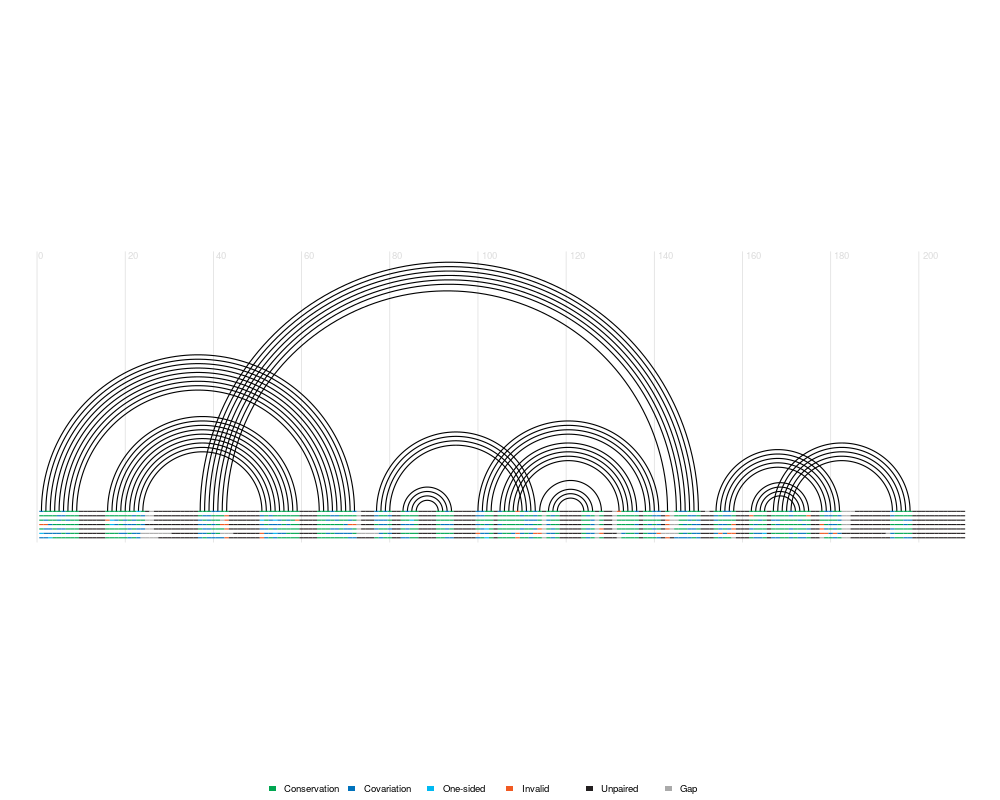
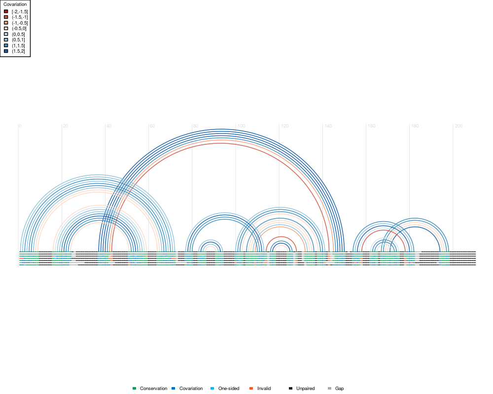
Plot nucleotide sequence coloured by covarianceDescriptionGiven a multiple sequence alignment and a corresponding secondary structure, nucleotides in the sequence alignment will be coloured according to the basepairing and conservation status, where green is the most commonly observed valid basepair in the column, dark blue being valid covariation (i.e. mutation into another valid basepair), cyan is one-sided mutation that retains the basepair, and red is a mutation where the basepair has been lost. Usage
    plotCovariance(msa, helix, arcs = TRUE, add = FALSE, grid = FALSE, text =
        FALSE, legend = TRUE, species = 0, base.colour = FALSE, palette = NA, flip =
        FALSE, grid.col = "white", grid.lwd = 0, text.cex = 0.5, text.col = "white",
        text.font = 2, text.family = "sans", species.cex = 0.5, species.col = "black",
        species.font = 2, species.family = "mono", shape = "circle", conflict.cutoff =
        0.01, conflict.lty = 2, conflict.col = NA, pad = c(0, 0, 0, 0), y = 0, x = 0,
        ...)
    plotDoubleCovariance(top.helix, bot.helix, top.msa, bot.msa = top.msa,
        add = FALSE, grid = FALSE, species = 0, legend = TRUE,
        pad = c(0, 0, 0, 0), ...)
    plotOverlapCovariance(predict.helix, known.helix, msa, bot.msa = TRUE,
        overlap.cutoff = 1, miss = "black", add = FALSE, grid = FALSE, species = 0,
        legend = TRUE, pad = c(0, 0, 0, 0), ...)
Arguments
ValueNot intended to return a value, will plot to GUI or file if specific. Author(s)Daniel Lai See Also
Examples
data(helix)
# Basic covariance plot
plotCovariance(fasta, known, cex = 0.8, lwd = 1.5)
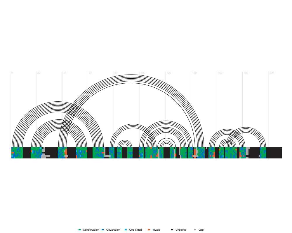
# Grid mode
plotCovariance(fasta, known, grid = TRUE, text = FALSE, cex = 0.8)
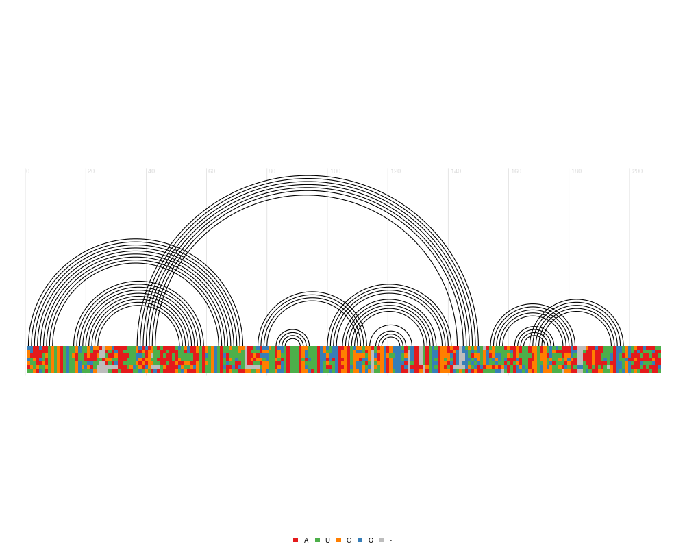
# Global style and nucleotide colouring
plotCovariance(fasta, known, grid = TRUE, text = FALSE, base.colour = TRUE)
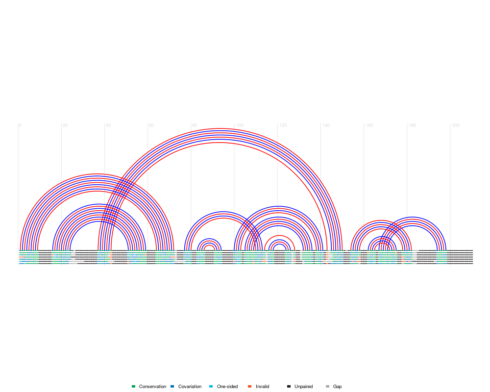
# Styling indivual helices with styling columns
known$col <- c("red", "blue")
plotCovariance(fasta, known, lwd = 2, cex = 0.8)
# Use in combination with colourBy functions
cov <- colourByCovariation(known, fasta, get = TRUE)
plotCovariance(fasta, cov)
legend("topleft", legend = attr(cov, "legend"),
fill = attr(cov, "fill"), title = "Covariation")
Results
R version 3.3.1 (2016-06-21) -- "Bug in Your Hair"
Copyright (C) 2016 The R Foundation for Statistical Computing
Platform: x86_64-pc-linux-gnu (64-bit)

R is free software and comes with ABSOLUTELY NO WARRANTY.
You are welcome to redistribute it under certain conditions.
Type 'license()' or 'licence()' for distribution details.

R is a collaborative project with many contributors.
Type 'contributors()' for more information and
'citation()' on how to cite R or R packages in publications.

Type 'demo()' for some demos, 'help()' for on-line help, or
'help.start()' for an HTML browser interface to help.
Type 'q()' to quit R.

> library(R4RNA)
Loading required package: Biostrings
Loading required package: BiocGenerics
Loading required package: parallel

Attaching package: 'BiocGenerics'

The following objects are masked from 'package:parallel':

    clusterApply, clusterApplyLB, clusterCall, clusterEvalQ,
    clusterExport, clusterMap, parApply, parCapply, parLapply,
    parLapplyLB, parRapply, parSapply, parSapplyLB

The following objects are masked from 'package:stats':

    IQR, mad, xtabs

The following objects are masked from 'package:base':

    Filter, Find, Map, Position, Reduce, anyDuplicated, append,
    as.data.frame, cbind, colnames, do.call, duplicated, eval, evalq,
    get, grep, grepl, intersect, is.unsorted, lapply, lengths, mapply,
    match, mget, order, paste, pmax, pmax.int, pmin, pmin.int, rank,
    rbind, rownames, sapply, setdiff, sort, table, tapply, union,
    unique, unsplit

Loading required package: S4Vectors
Loading required package: stats4

Attaching package: 'S4Vectors'

The following objects are masked from 'package:base':

    colMeans, colSums, expand.grid, rowMeans, rowSums

Loading required package: IRanges
Loading required package: XVector
> png(filename="/home/ddbj/snapshot/RGM3/R_BC/result/R4RNA/plotCovariance.Rd_%03d_medium.png", width=480, height=480)
> ### Name: Covariation Plots
> ### Title: Plot nucleotide sequence coloured by covariance
> ### Aliases: plotCovariance plotDoubleCovariance plotOverlapCovariance
> ### Keywords: aplot
>
> ### ** Examples
>
>     data(helix)
>
>     # Basic covariance plot
>     plotCovariance(fasta, known, cex = 0.8, lwd = 1.5)
>
>     # Grid mode
>     plotCovariance(fasta, known, grid = TRUE, text = FALSE, cex = 0.8)
>
>     # Global style and nucleotide colouring
>     plotCovariance(fasta, known, grid = TRUE, text = FALSE, base.colour = TRUE)
>
>     # Styling indivual helices with styling columns
>     known$col <- c("red", "blue")
>     plotCovariance(fasta, known, lwd = 2, cex = 0.8)
>
>     # Use in combination with colourBy functions
>     cov <- colourByCovariation(known, fasta, get = TRUE)
>     plotCovariance(fasta, cov)
>     legend("topleft", legend = attr(cov, "legend"),
+         fill = attr(cov, "fill"), title = "Covariation")
>
>
>
>
>
>
> dev.off()
null device
          1
>
|