Supported by Dr. Osamu Ogasawara and  . . |
|
Last data update: 2014.03.03 |
Visualization of biological relationshipsDescription
Usage
  plot2D(object,...)

  ## S4 method for signature 'DAVIDResult'
plot2D(object, dataFrame)

  ## S4 method for signature 'DAVIDFunctionalAnnotationChart'
plot2D(object,color=c("FALSE"="black",
  "TRUE"="green"))

  ## S4 method for signature 'DAVIDGeneCluster'
plot2D(object,color=c("FALSE"="black","TRUE"="green"),names=FALSE)

  ## S4 method for signature 'DAVIDTermCluster'
plot2D(object,number=1,color=c("FALSE"="black","TRUE"=
  "green"))

  ## S4 method for signature 'DAVIDFunctionalAnnotationTable'
plot2D(object,
  category, id, names.genes=FALSE,
  names.category=FALSE,color=c("FALSE"="black","TRUE"="green"))
Arguments
Valuea ggplot object if the object is not empty. Author(s)Cristobal Fresno and Elmer A Fernandez See AlsoOther DAVIDFunctionalAnnotationChart:
Other DAVIDFunctionalAnnotationTable:
Other DAVIDGeneCluster:
Other DAVIDResult: Other DAVIDTermCluster:
Examples
{
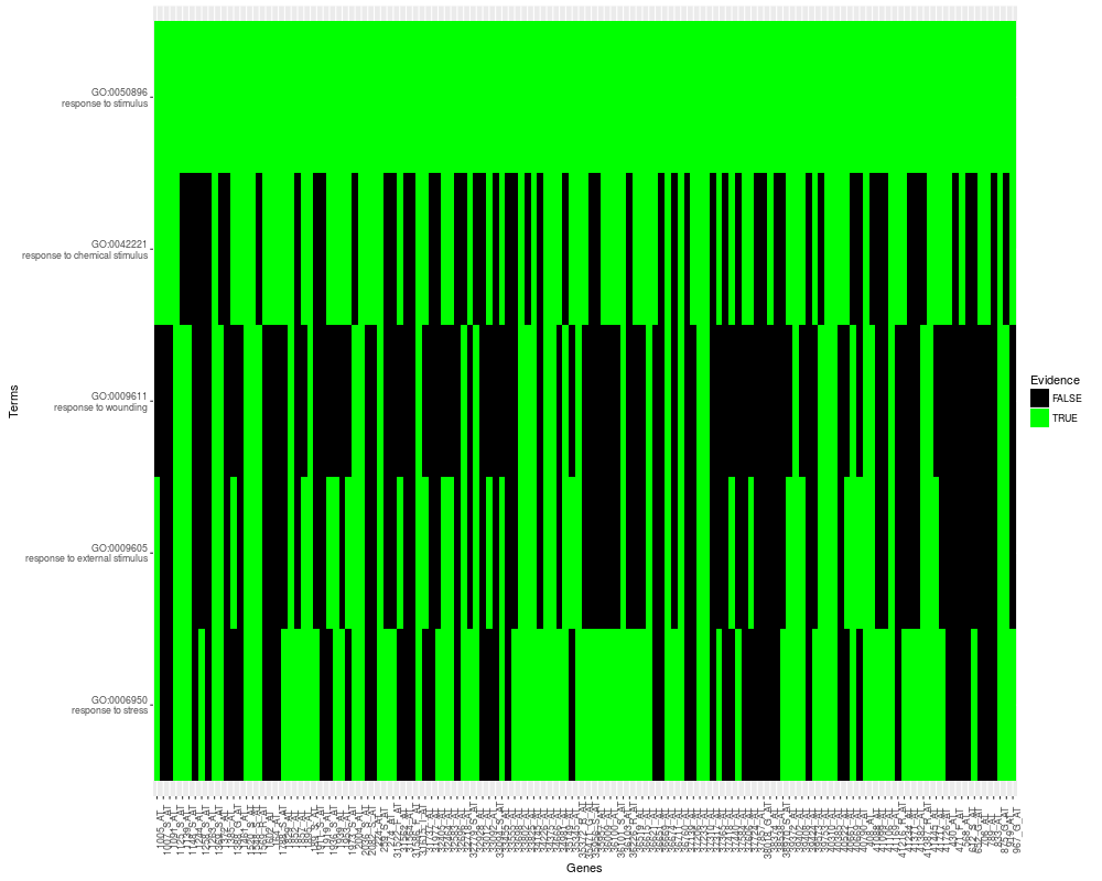
##DAVIDFunctionalAnnotationChart example:
##Load the Functional Annotation Chart file report for the input demo
##file 2, using data function. Just to keep it simple, for the first five
##terms present in funChart2 object, create a DAVIDFunctionalAnnotationChart
##object and plot a 2D tile matrix with the reported evidence (green) or not
##(black).
data(funChart2)
plot2D(DAVIDFunctionalAnnotationChart(funChart2[1:5, ]),
color=c("FALSE"="black", "TRUE"="green"))
##DAVIDFunctionalAnnotationTable example
##Load the Functional Annotation Table file report for the input demo
##file 1, using data function. Then, create a DAVIDFunctionalAnnotationTable
##object using the loaded data.frame annotationTable1.
data(annotationTable1)
davidFunTable1<-DAVIDFunctionalAnnotationTable(annotationTable1)
##Plot the membership of only for the first six terms in this
##category, with only the genes of the first six terms with at least one
##evidence code.
##Category filtering...
categorySelection<-list(head(dictionary(davidFunTable1,
categories(davidFunTable1)[1])$ID))
names(categorySelection)<-categories(davidFunTable1)[1]
##Gene filter...
id<-membership(davidFunTable1, categories(davidFunTable1)[1])[,1:6]
id<-ids(genes(davidFunTable1))[rowSums(id)>0]
##Finally the membership tile plot
plot2D(davidFunTable1, category=categorySelection, id=id,
names.category=TRUE)
##DAVIDGeneCluster example:
##Load the Gene Functional Classification Tool file report for the
##input demo list 1 file to create a DAVIDGeneCluster object.
setwd(tempdir())
fileName<-system.file("files/geneClusterReport1.tab.tar.gz",
package="RDAVIDWebService")
untar(fileName)
davidGeneCluster1<-DAVIDGeneCluster(untar(fileName, list=TRUE))
##We can inspect a 2D tile membership plot, to visual inspect for
##overlapping of genes across the clusters. Or use an scaled version of gene
##names to see the association of gene cluster, e.g., cluster 3 is related to
##ATP genes.
plot2D(davidGeneCluster1)
plot2D(davidGeneCluster1,names=TRUE)+
theme(axis.text.y=element_text(size=rel(0.9)))
##DAVIDTermCluster example:
##Load the Gene Functional Classification Tool file report for the
##input demo file 2 to create a DAVIDGeneCluster object.
setwd(tempdir())
fileName<-system.file("files/termClusterReport2.tab.tar.gz",
package="RDAVIDWebService")
untar(fileName)
davidTermCluster2<-DAVIDTermCluster(untar(fileName, list=TRUE))
##Finally, we can inspect a 2D tile membership plot, to visual inspect for
##overlapping of genes across the term members of the selected cluster,
##e.g., the first cluster .
plot2D(davidTermCluster2, number=1)
}
Results
R version 3.3.1 (2016-06-21) -- "Bug in Your Hair"
Copyright (C) 2016 The R Foundation for Statistical Computing
Platform: x86_64-pc-linux-gnu (64-bit)

R is free software and comes with ABSOLUTELY NO WARRANTY.
You are welcome to redistribute it under certain conditions.
Type 'license()' or 'licence()' for distribution details.

R is a collaborative project with many contributors.
Type 'contributors()' for more information and
'citation()' on how to cite R or R packages in publications.

Type 'demo()' for some demos, 'help()' for on-line help, or
'help.start()' for an HTML browser interface to help.
Type 'q()' to quit R.

> library(RDAVIDWebService)
Loading required package: graph
Loading required package: BiocGenerics
Loading required package: parallel

Attaching package: 'BiocGenerics'

The following objects are masked from 'package:parallel':

    clusterApply, clusterApplyLB, clusterCall, clusterEvalQ,
    clusterExport, clusterMap, parApply, parCapply, parLapply,
    parLapplyLB, parRapply, parSapply, parSapplyLB

The following objects are masked from 'package:stats':

    IQR, mad, xtabs

The following objects are masked from 'package:base':

    Filter, Find, Map, Position, Reduce, anyDuplicated, append,
    as.data.frame, cbind, colnames, do.call, duplicated, eval, evalq,
    get, grep, grepl, intersect, is.unsorted, lapply, lengths, mapply,
    match, mget, order, paste, pmax, pmax.int, pmin, pmin.int, rank,
    rbind, rownames, sapply, setdiff, sort, table, tapply, union,
    unique, unsplit

Loading required package: GOstats
Loading required package: Biobase
Welcome to Bioconductor

    Vignettes contain introductory material; view with
    'browseVignettes()'. To cite Bioconductor, see
    'citation("Biobase")', and for packages 'citation("pkgname")'.

Loading required package: Category
Loading required package: stats4
Loading required package: AnnotationDbi
Loading required package: IRanges
Loading required package: S4Vectors

Attaching package: 'S4Vectors'

The following objects are masked from 'package:base':

    colMeans, colSums, expand.grid, rowMeans, rowSums

Loading required package: Matrix

Attaching package: 'Matrix'

The following object is masked from 'package:S4Vectors':

    expand


Attaching package: 'GOstats'

The following object is masked from 'package:AnnotationDbi':

    makeGOGraph

Loading required package: ggplot2

Attaching package: 'RDAVIDWebService'

The following object is masked from 'package:AnnotationDbi':

    species

The following object is masked from 'package:IRanges':

    members

The following objects are masked from 'package:BiocGenerics':

    counts, species

> png(filename="/home/ddbj/snapshot/RGM3/R_BC/result/RDAVIDWebService/DAVIDClasses-plot2D.Rd_%03d_medium.png", width=480, height=480)
> ### Name: plot2D
> ### Title: Visualization of biological relationships
> ### Aliases: plot2D,DAVIDFunctionalAnnotationChart-method
> ###   plot2D,DAVIDFunctionalAnnotationTable-method
> ###   plot2D,DAVIDGeneCluster-method plot2D,DAVIDResult-method
> ###   plot2D,DAVIDTermCluster-method plot2D-methods plot2D
>
> ### ** Examples
>
> {
+ ##DAVIDFunctionalAnnotationChart example:
+ ##Load the Functional Annotation Chart file report for the input demo
+ ##file 2, using data function. Just to keep it simple, for the first five
+ ##terms present in funChart2 object, create a DAVIDFunctionalAnnotationChart
+ ##object and plot a 2D tile matrix with the reported evidence (green) or not
+ ##(black).
+ data(funChart2)
+ plot2D(DAVIDFunctionalAnnotationChart(funChart2[1:5, ]),
+ color=c("FALSE"="black", "TRUE"="green"))
+
+ ##DAVIDFunctionalAnnotationTable example
+ ##Load the Functional Annotation Table file report for the input demo
+ ##file 1, using data function. Then, create a DAVIDFunctionalAnnotationTable
+ ##object using the loaded data.frame annotationTable1.
+ data(annotationTable1)
+ davidFunTable1<-DAVIDFunctionalAnnotationTable(annotationTable1)
+
+ ##Plot the membership of only for the first six terms in this
+ ##category, with only the genes of the first six terms with at least one
+ ##evidence code.
+ ##Category filtering...
+ categorySelection<-list(head(dictionary(davidFunTable1,
+ categories(davidFunTable1)[1])$ID))
+ names(categorySelection)<-categories(davidFunTable1)[1]
+
+ ##Gene filter...
+ id<-membership(davidFunTable1, categories(davidFunTable1)[1])[,1:6]
+ id<-ids(genes(davidFunTable1))[rowSums(id)>0]
+
+ ##Finally the membership tile plot
+ plot2D(davidFunTable1, category=categorySelection, id=id,
+ names.category=TRUE)
+
+ ##DAVIDGeneCluster example:
+ ##Load the Gene Functional Classification Tool file report for the
+ ##input demo list 1 file to create a DAVIDGeneCluster object.
+ setwd(tempdir())
+ fileName<-system.file("files/geneClusterReport1.tab.tar.gz",
+ package="RDAVIDWebService")
+ untar(fileName)
+ davidGeneCluster1<-DAVIDGeneCluster(untar(fileName, list=TRUE))
+
+ ##We can inspect a 2D tile membership plot, to visual inspect for
+ ##overlapping of genes across the clusters. Or use an scaled version of gene
+ ##names to see the association of gene cluster, e.g., cluster 3 is related to
+ ##ATP genes.
+ plot2D(davidGeneCluster1)
+ plot2D(davidGeneCluster1,names=TRUE)+
+ theme(axis.text.y=element_text(size=rel(0.9)))
+
+ ##DAVIDTermCluster example:
+ ##Load the Gene Functional Classification Tool file report for the
+ ##input demo file 2 to create a DAVIDGeneCluster object.
+ setwd(tempdir())
+ fileName<-system.file("files/termClusterReport2.tab.tar.gz",
+ package="RDAVIDWebService")
+ untar(fileName)
+ davidTermCluster2<-DAVIDTermCluster(untar(fileName, list=TRUE))
+
+ ##Finally, we can inspect a 2D tile membership plot, to visual inspect for
+ ##overlapping of genes across the term members of the selected cluster,
+ ##e.g., the first cluster .
+ plot2D(davidTermCluster2, number=1)
+ }
>
>
>
>
>
> dev.off()
null device
          1
>
|