R Graphical Manual

Browse All

Last data update: 2014.03.03

R: Expectation conditional maximization of negative binomial HMM...

nbh_em

R Documentation

Expectation conditional maximization of negative binomial HMM parameters using forward-backward algorithm

Description

Given an input read count vector of integers, the function optimizes the parameters for the negative binomial HMM of K hidden states using expectation conditional maximization with forward-backward algorithm to acheive the exact inference.

Usage

nbh_em(count, TRANS, alpha, beta, NBH_NIT_MAX = 250, 
	NBH_TOL = 1e-05, MAXALPHA = 1e+07, MAXBETA = 1e+07)

Arguments

`count`	A vector of integers, conceptaully representative of the read counts within bins of chromosome.
`TRANS`	Transition probability matrix, a squared matrix of probabilities (0 ≤ p ≤ 1) with row and column length equal to that of alpha and beta and row sum and column sum both equal to 1 (within some numerical deviation of 1e-6).
`alpha`	Shape parameter of the NB as a vector of positive values with length equal to that of beta and the row/column of TRANS.
`beta`	Inverse scale parameter of the NB as a vector of positive values with length equal to that of beta and the row/column of TRANS.
`NBH_NIT_MAX`	Maximum number of EM iterations (Default: 250) for the negative binomial hidden Markov model (NBH).
`NBH_TOL`	Threshold as fraction of increase in likelihood (given the current NBH parameters) comparing with the likelihood from the last iteration. EM for the NBH stops when the improvement is below the threshold (Default: 0.001).
`MAXALPHA`	The maximum value of alpha in case the update goes beyond the numerical upper limit of the system. Once alpha becomes larger than `MAXALPHA`, the EM itaration is prematurely terminated to prevent malfunction.
`MAXBETA`	The maximum value of beta in case the update goes beyond the numerical upper limit of the system. Once beta becomes larger than `MAXBETA`, the EM itaration is prematurely terminated to prevent malfunction.

Details

Given a K-state HMM with NB emission (NBH), the goal is to maximize the likelihood function with respect to the parameters comprising of α_k and β_k for the K NB components and the transition probabilities A_jk between any state j and k, which are the priors p(z=k). Because there is no analytical solution for the maximum likelihood (ML) estimators of the above quantities, a modified EM procedures called Expectation Conditional Maximization is employed (Meng and Rubin, 1994).

In E-step, the posterior probability is evaluated by forward-backward algorithm using NB density functions with initialized alpha, beta, and TRANS. In the CM step, A_jk is evaluated first followed by Newton updates of α_k and β_k. EM iteration terminates when the percetnage of increase of log likelihood drop below NBH_TOL, which is deterministic since EM is guaranteed to converge. For more details, please see the manuscript of RIPSeeker.

Value

A list containing:

`alpha`	optimized alpha_k for NB at state K
`beta`	optimized beta_k for NB at state K
`TRANS`	optimized transition probability matrix
`logl`	Log likelihood in each EM iteration.
`postprob`	Posterior probabilities for each observed data point at the last EM iteration.
`dens`	the negative binomial probabilities computed at the last EM iteration

Author(s)

Yue Li

References

Rabiner, L. R. (1989). A tutorial on hidden Markov models and selected applications in speech recognition (Vol. 77, pp. 257-286). Presented at the Proceedings of the IEEE. doi:10.1109/5.18626

Christopher Bishop. Pattern recognition and machine learning. Number 605-631 in Information Science and Statisitcs. Springer Science, 2006.

X. L. Meng, D. B. Rubin, Maximum likelihood estimation via the ECM algorithm: A general framework, Biometrika, 80(2):267-278 (1993).

J. A. Fessler, A. O. Hero, Space-alternating generalized expectation-maximization algorithm, IEEE Tr. on Signal Processing, 42(10):2664 -2677 (1994).

Capp'e, O. (2001). H2M : A set of MATLAB/OCTAVE functions for the EM estimation of mixtures and hidden Markov models. (http://perso.telecom-paristech.fr/cappe/h2m/)

Examples

# Simulate data
TRANS_s <- matrix(c(0.9, 0.1, 0.3, 0.7), nrow=2, byrow=TRUE)
alpha_s <- c(2, 4)
beta_s  <- c(1, 0.25)
Total <- 100

x <- nbh_gen(TRANS_s, alpha_s, beta_s, Total);

count <- x$count
label <- x$label

Total <- length(count)

# dummy initialization
TRANS0 <- matrix(rep(0.5,4), 2)

alpha0 <- c(1, 20)

beta0 <- c(1, 1)

NIT_MAX <- 50
TOL <- 1e-100
nbh <- nbh_em(count, TRANS0, alpha0, beta0, NIT_MAX, TOL)

map.accuracy <- length(which(max.col(nbh$postprob) == label))/Total

vit <- nbh_vit(count, nbh$TRANS, nbh$alpha, nbh$beta)

vit.accuracy <- length(which(vit$class == label))/Total

# Plots
par(mfrow=c(2,2), cex.lab=1.2, cex.main=1.2)

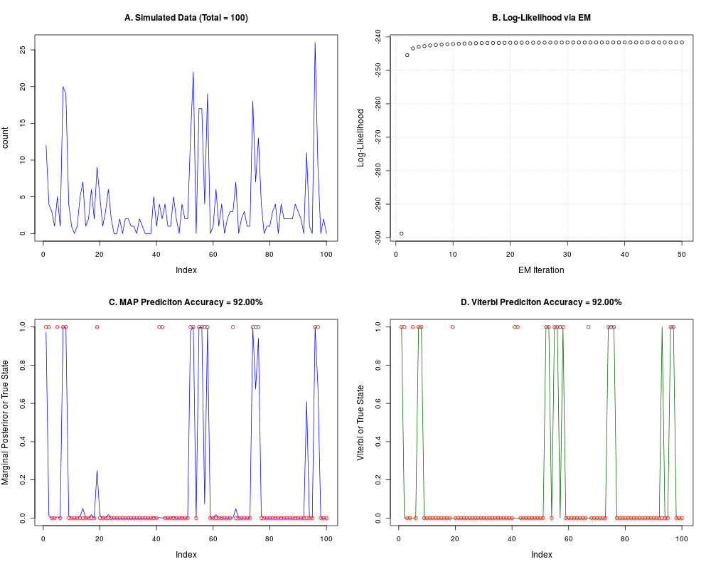
plot(count, col="blue", type="l", main=sprintf("A. Simulated Data (Total = %i)",Total))

plot(as.numeric(nbh$logl), xlab="EM Iteration", ylab="Log-Likelihood", 
main="B. Log-Likelihood via EM");grid()


# Marginal postprob
plot(nbh$postprob[,2], col="blue", type="l", ylim = c(0,1),
ylab="Marginal Posteriror or True State")
points(label-1, col="red")
title(main = sprintf("C. MAP Prediciton Accuracy = %.2f%s", 100 * map.accuracy, "%"))


# Viterbi states
plot(vit$class - 1, col="dark green", type="l", ylim = c(0,1),
ylab="Viterbi or True State")
points(label-1, col="red")
title(main = sprintf("D. Viterbi Prediciton Accuracy = %.2f%s", 100 * vit.accuracy, "%"))

Results


R version 3.3.1 (2016-06-21) -- "Bug in Your Hair"
Copyright (C) 2016 The R Foundation for Statistical Computing
Platform: x86_64-pc-linux-gnu (64-bit)

R is free software and comes with ABSOLUTELY NO WARRANTY.
You are welcome to redistribute it under certain conditions.
Type 'license()' or 'licence()' for distribution details.

R is a collaborative project with many contributors.
Type 'contributors()' for more information and
'citation()' on how to cite R or R packages in publications.

Type 'demo()' for some demos, 'help()' for on-line help, or
'help.start()' for an HTML browser interface to help.
Type 'q()' to quit R.

> library(RIPSeeker)
Loading required package: S4Vectors
Loading required package: stats4
Loading required package: BiocGenerics
Loading required package: parallel

Attaching package: 'BiocGenerics'

The following objects are masked from 'package:parallel':

    clusterApply, clusterApplyLB, clusterCall, clusterEvalQ,
    clusterExport, clusterMap, parApply, parCapply, parLapply,
    parLapplyLB, parRapply, parSapply, parSapplyLB

The following objects are masked from 'package:stats':

    IQR, mad, xtabs

The following objects are masked from 'package:base':

    Filter, Find, Map, Position, Reduce, anyDuplicated, append,
    as.data.frame, cbind, colnames, do.call, duplicated, eval, evalq,
    get, grep, grepl, intersect, is.unsorted, lapply, lengths, mapply,
    match, mget, order, paste, pmax, pmax.int, pmin, pmin.int, rank,
    rbind, rownames, sapply, setdiff, sort, table, tapply, union,
    unique, unsplit


Attaching package: 'S4Vectors'

The following objects are masked from 'package:base':

    colMeans, colSums, expand.grid, rowMeans, rowSums

Loading required package: IRanges
Loading required package: GenomicRanges
Loading required package: GenomeInfoDb
Loading required package: SummarizedExperiment
Loading required package: Biobase
Welcome to Bioconductor

    Vignettes contain introductory material; view with
    'browseVignettes()'. To cite Bioconductor, see
    'citation("Biobase")', and for packages 'citation("pkgname")'.

Loading required package: Rsamtools
Loading required package: Biostrings
Loading required package: XVector
Loading required package: GenomicAlignments
Loading required package: rtracklayer
> png(filename="/home/ddbj/snapshot/RGM3/R_BC/result/RIPSeeker/nbh_em.Rd_%03d_medium.png", width=480, height=480)
> ### Name: nbh_em
> ### Title: Expectation conditional maximization of negative binomial HMM
> ###   parameters using forward-backward algorithm
> ### Aliases: nbh_em
> 
> ### ** Examples
> 
> # Simulate data
> TRANS_s <- matrix(c(0.9, 0.1, 0.3, 0.7), nrow=2, byrow=TRUE)
> alpha_s <- c(2, 4)
> beta_s  <- c(1, 0.25)
> Total <- 100
> 
> x <- nbh_gen(TRANS_s, alpha_s, beta_s, Total);
> 
> count <- x$count
> label <- x$label
> 
> Total <- length(count)
> 
> # dummy initialization
> TRANS0 <- matrix(rep(0.5,4), 2)
> 
> alpha0 <- c(1, 20)
> 
> beta0 <- c(1, 1)
> 
> NIT_MAX <- 50
> TOL <- 1e-100
> nbh <- nbh_em(count, TRANS0, alpha0, beta0, NIT_MAX, TOL)
Iteration 0:	-313.917
Iteration 1:	-272.103
Iteration 2:	-270.678
Iteration 3:	-270.271
Iteration 4:	-270.008
Iteration 5:	-269.789
Iteration 6:	-269.600
Iteration 7:	-269.434
Iteration 8:	-269.289
Iteration 9:	-269.159
Iteration 10:	-269.041
Iteration 11:	-268.934
Iteration 12:	-268.836
Iteration 13:	-268.745
Iteration 14:	-268.659
Iteration 15:	-268.579
Iteration 16:	-268.503
Iteration 17:	-268.430
Iteration 18:	-268.360
Iteration 19:	-268.294
Iteration 20:	-268.229
Iteration 21:	-268.167
Iteration 22:	-268.107
Iteration 23:	-268.048
Iteration 24:	-267.991
Iteration 25:	-267.936
Iteration 26:	-267.882
Iteration 27:	-267.829
Iteration 28:	-267.778
Iteration 29:	-267.728
Iteration 30:	-267.678
Iteration 31:	-267.631
Iteration 32:	-267.584
Iteration 33:	-267.538
Iteration 34:	-267.493
Iteration 35:	-267.450
Iteration 36:	-267.407
Iteration 37:	-267.366
Iteration 38:	-267.325
Iteration 39:	-267.286
Iteration 40:	-267.247
Iteration 41:	-267.210
Iteration 42:	-267.173
Iteration 43:	-267.138
Iteration 44:	-267.103
Iteration 45:	-267.070
Iteration 46:	-267.037
Iteration 47:	-267.005
Iteration 48:	-266.975
Iteration 49:	-266.945
> 
> map.accuracy <- length(which(max.col(nbh$postprob) == label))/Total
> 
> vit <- nbh_vit(count, nbh$TRANS, nbh$alpha, nbh$beta)
> 
> vit.accuracy <- length(which(vit$class == label))/Total
> 
> # Plots
> par(mfrow=c(2,2), cex.lab=1.2, cex.main=1.2)
> 
> plot(count, col="blue", type="l", main=sprintf("A. Simulated Data (Total = %i)",Total))
> 
> plot(as.numeric(nbh$logl), xlab="EM Iteration", ylab="Log-Likelihood", 
+ main="B. Log-Likelihood via EM");grid()
> 
> 
> # Marginal postprob
> plot(nbh$postprob[,2], col="blue", type="l", ylim = c(0,1),
+ ylab="Marginal Posteriror or True State")
> points(label-1, col="red")
> title(main = sprintf("C. MAP Prediciton Accuracy = %.2f%s", 100 * map.accuracy, "%"))
> 
> 
> # Viterbi states
> plot(vit$class - 1, col="dark green", type="l", ylim = c(0,1),
+ ylab="Viterbi or True State")
> points(label-1, col="red")
> title(main = sprintf("D. Viterbi Prediciton Accuracy = %.2f%s", 100 * vit.accuracy, "%"))
> 
> 		
> 
> 
> 
> 
> 
> dev.off()
null device 
          1 
>