Supported by Dr. Osamu Ogasawara and  . . |
|
Last data update: 2014.03.03 |
Derive maximum likelihood hidden state sequence using Viterbi algorithmDescriptionGiven read counts and HMM parameters (optimized by Usagenbh_vit(count, TRANS, alpha, beta) Arguments
DetailsGiven a K-state HMM with NB emission (NBH), the goal is to find the latent states corresponding to the observed data that maximize the joint likelihood ln p(X, Z) = ln p(x_1, …, x_N, z_1, …, z_N). The optimal solution is obtained via Viterbi algorithm, which essentially belongs to the more general framework of Dynamic Programming. Briefly, starting from the second node of the Markov chain, we select state of the first node that maximizes ln p(x_1, x_2, z_2 | z_1) for every state of z_2. Then, we move on to the next node and the next until reaching to the last node. In the end, we make choice for the state of the last node that together leads to the maximum ln p(X, Z). Finally, we backtrack to find the choices of states in all of the intermeidate nodes to form the final solution. ValueA list containing:
NoteThe function is expected to run after learning the model parameters of HMM using Author(s)Yue Li ReferencesRabiner, L. R. (1989). A tutorial on hidden Markov models and selected applications in speech recognition (Vol. 77, pp. 257-286). Presented at the Proceedings of the IEEE. doi:10.1109/5.18626 Christopher Bishop. Pattern recognition and machine learning. Number 605-631 in Information Science and Statisitcs. Springer Science, 2006. X. L. Meng, D. B. Rubin, Maximum likelihood estimation via the ECM algorithm: A general framework, Biometrika, 80(2):267-278 (1993). J. A. Fessler, A. O. Hero, Space-alternating generalized expectation-maximization algorithm, IEEE Tr. on Signal Processing, 42(10):2664 -2677 (1994). Capp'e, O. (2001). H2M : A set of MATLAB/OCTAVE functions for the EM estimation of mixtures and hidden Markov models. (http://perso.telecom-paristech.fr/cappe/h2m/) See Also
Examples
# Simulate data
TRANS_s <- matrix(c(0.9, 0.1, 0.3, 0.7), nrow=2, byrow=TRUE)
alpha_s <- c(2, 4)
beta_s <- c(1, 0.25)
Total <- 100
x <- nbh_gen(TRANS_s, alpha_s, beta_s, Total);
count <- x$count
label <- x$label
Total <- length(count)
# dummy initialization
TRANS0 <- matrix(rep(0.5,4), 2)
alpha0 <- c(1, 20)
beta0 <- c(1, 1)
NIT_MAX <- 50
TOL <- 1e-100
nbh <- nbh_em(count, TRANS0, alpha0, beta0, NIT_MAX, TOL)
map.accuracy <- length(which(max.col(nbh$postprob) == label))/Total
vit <- nbh_vit(count, nbh$TRANS, nbh$alpha, nbh$beta)
vit.accuracy <- length(which(vit$class == label))/Total
# Plots
par(mfrow=c(2,2), cex.lab=1.2, cex.main=1.2)
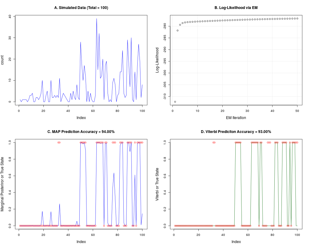
plot(count, col="blue", type="l", main=sprintf("A. Simulated Data (Total = %i)",Total))
plot(as.numeric(nbh$logl), xlab="EM Iteration", ylab="Log-Likelihood",
main="B. Log-Likelihood via EM");grid()
# Marginal postprob
plot(nbh$postprob[,2], col="blue", type="l", ylim = c(0,1),
ylab="Marginal Posteriror or True State")
points(label-1, col="red")
title(main = sprintf("C. MAP Prediciton Accuracy = %.2f%s", 100 * map.accuracy, "%"))
# Viterbi states
plot(vit$class - 1, col="dark green", type="l", ylim = c(0,1),
ylab="Viterbi or True State")
points(label-1, col="red")
title(main = sprintf("D. Viterbi Prediciton Accuracy = %.2f%s", 100 * vit.accuracy, "%"))
Results
R version 3.3.1 (2016-06-21) -- "Bug in Your Hair"
Copyright (C) 2016 The R Foundation for Statistical Computing
Platform: x86_64-pc-linux-gnu (64-bit)

R is free software and comes with ABSOLUTELY NO WARRANTY.
You are welcome to redistribute it under certain conditions.
Type 'license()' or 'licence()' for distribution details.

R is a collaborative project with many contributors.
Type 'contributors()' for more information and
'citation()' on how to cite R or R packages in publications.

Type 'demo()' for some demos, 'help()' for on-line help, or
'help.start()' for an HTML browser interface to help.
Type 'q()' to quit R.

> library(RIPSeeker)
Loading required package: S4Vectors
Loading required package: stats4
Loading required package: BiocGenerics
Loading required package: parallel

Attaching package: 'BiocGenerics'

The following objects are masked from 'package:parallel':

    clusterApply, clusterApplyLB, clusterCall, clusterEvalQ,
    clusterExport, clusterMap, parApply, parCapply, parLapply,
    parLapplyLB, parRapply, parSapply, parSapplyLB

The following objects are masked from 'package:stats':

    IQR, mad, xtabs

The following objects are masked from 'package:base':

    Filter, Find, Map, Position, Reduce, anyDuplicated, append,
    as.data.frame, cbind, colnames, do.call, duplicated, eval, evalq,
    get, grep, grepl, intersect, is.unsorted, lapply, lengths, mapply,
    match, mget, order, paste, pmax, pmax.int, pmin, pmin.int, rank,
    rbind, rownames, sapply, setdiff, sort, table, tapply, union,
    unique, unsplit


Attaching package: 'S4Vectors'

The following objects are masked from 'package:base':

    colMeans, colSums, expand.grid, rowMeans, rowSums

Loading required package: IRanges
Loading required package: GenomicRanges
Loading required package: GenomeInfoDb
Loading required package: SummarizedExperiment
Loading required package: Biobase
Welcome to Bioconductor

    Vignettes contain introductory material; view with
    'browseVignettes()'. To cite Bioconductor, see
    'citation("Biobase")', and for packages 'citation("pkgname")'.

Loading required package: Rsamtools
Loading required package: Biostrings
Loading required package: XVector
Loading required package: GenomicAlignments
Loading required package: rtracklayer
> png(filename="/home/ddbj/snapshot/RGM3/R_BC/result/RIPSeeker/nbh_vit.Rd_%03d_medium.png", width=480, height=480)
> ### Name: nbh_vit
> ### Title: Derive maximum likelihood hidden state sequence using Viterbi
> ###   algorithm
> ### Aliases: nbh_vit
>
> ### ** Examples
>
> # Simulate data
> TRANS_s <- matrix(c(0.9, 0.1, 0.3, 0.7), nrow=2, byrow=TRUE)
> alpha_s <- c(2, 4)
> beta_s  <- c(1, 0.25)
> Total <- 100
>
> x <- nbh_gen(TRANS_s, alpha_s, beta_s, Total);
>
> count <- x$count
> label <- x$label
>
> Total <- length(count)
>
> # dummy initialization
> TRANS0 <- matrix(rep(0.5,4), 2)
>
> alpha0 <- c(1, 20)
>
> beta0 <- c(1, 1)
>
> NIT_MAX <- 50
> TOL <- 1e-100
> nbh <- nbh_em(count, TRANS0, alpha0, beta0, NIT_MAX, TOL)
Iteration 0:	-320.885
Iteration 1:	-285.571
Iteration 2:	-284.162
Iteration 3:	-283.800
Iteration 4:	-283.484
Iteration 5:	-283.196
Iteration 6:	-282.929
Iteration 7:	-282.679
Iteration 8:	-282.442
Iteration 9:	-282.215
Iteration 10:	-281.997
Iteration 11:	-281.787
Iteration 12:	-281.584
Iteration 13:	-281.388
Iteration 14:	-281.198
Iteration 15:	-281.013
Iteration 16:	-280.834
Iteration 17:	-280.661
Iteration 18:	-280.493
Iteration 19:	-280.330
Iteration 20:	-280.173
Iteration 21:	-280.021
Iteration 22:	-279.874
Iteration 23:	-279.733
Iteration 24:	-279.597
Iteration 25:	-279.466
Iteration 26:	-279.341
Iteration 27:	-279.221
Iteration 28:	-279.106
Iteration 29:	-278.996
Iteration 30:	-278.891
Iteration 31:	-278.791
Iteration 32:	-278.695
Iteration 33:	-278.605
Iteration 34:	-278.519
Iteration 35:	-278.438
Iteration 36:	-278.361
Iteration 37:	-278.288
Iteration 38:	-278.220
Iteration 39:	-278.155
Iteration 40:	-278.094
Iteration 41:	-278.037
Iteration 42:	-277.984
Iteration 43:	-277.933
Iteration 44:	-277.886
Iteration 45:	-277.842
Iteration 46:	-277.801
Iteration 47:	-277.763
Iteration 48:	-277.727
Iteration 49:	-277.694
>
> map.accuracy <- length(which(max.col(nbh$postprob) == label))/Total
>
> vit <- nbh_vit(count, nbh$TRANS, nbh$alpha, nbh$beta)
>
> vit.accuracy <- length(which(vit$class == label))/Total
>
> # Plots
> par(mfrow=c(2,2), cex.lab=1.2, cex.main=1.2)
>
> plot(count, col="blue", type="l", main=sprintf("A. Simulated Data (Total = %i)",Total))
>
> plot(as.numeric(nbh$logl), xlab="EM Iteration", ylab="Log-Likelihood",
+ main="B. Log-Likelihood via EM");grid()
>
>
> # Marginal postprob
> plot(nbh$postprob[,2], col="blue", type="l", ylim = c(0,1),
+ ylab="Marginal Posteriror or True State")
> points(label-1, col="red")
> title(main = sprintf("C. MAP Prediciton Accuracy = %.2f%s", 100 * map.accuracy, "%"))
>
>
> # Viterbi states
> plot(vit$class - 1, col="dark green", type="l", ylim = c(0,1),
+ ylab="Viterbi or True State")
> points(label-1, col="red")
> title(main = sprintf("D. Viterbi Prediciton Accuracy = %.2f%s", 100 * vit.accuracy, "%"))
>
>
>
>
>
>
> dev.off()
null device
          1
>
|